Backhaus, Andreas (2018): Essays on development economics and economic history. Dissertation, LMU München: Volkswirtschaftliche Fakultät

(1)

Essays on Development Economics

and Economic History

Inaugural-Dissertation

zur Erlangung des Grades

Doctor oeconomiae publicae (Dr. oec. publ.)

an der Ludwig-Maximilians-Universität München

2017

vorgelegt von

Andreas Backhaus

Referent: Prof. Dr. Uwe Sunde

Korreferent: Prof. Dr. Ludger Wößmann

(2)

Datum der mündlichen Prüfung: 18.01.2018

(3)

Acknowledgements

First, I would like to thank Stephan Klasen and Gilles Saint-Paul, who recommended me for the PhD position in Munich. I am also much obliged to Dalia Marin, who made the initial decision to accept me into the MGSE.

Next, I would like to thank my primary supervisor Uwe Sunde, who accepted me as a member into the Chair for Population Economics. I particularly appreciate that he always encouraged every new line of my research without imposing how I pursue it. Being granted the freedom to try out and to learn was elementary to my doctoral studies that led up to this dissertation. I would further like to thank Ludger Wößmann, who agreed to act as my secondary supervisor, and Matteo Cervellati for serving as the oral examiner on my dissertation committee. Eva Tehua and Susan Fay were vital for mastering all administrative procedures in the background.

I am grateful for the opportunity to have worked with Inma Martinez-Zarzoso and Chris Muris on our joint paper. I would further like to express my gratitude towards Jan-Otmar Hesse, who kept my interest in the history of economic thought alive.

My fellow PhD students, in particular at the Chair of International Economics and the Chair for Population Economics, contributed significantly to my endurance and my motivation over the course of the years. In particular, I would like to thank my officemates Gerrit and Rainer, who made this episode much more fun than it would have been without them. Dina always encouraged both my interest in Central and Eastern Europe and my curiosity about hiking, both of which turned out to be beneficial for my PhD advancement and lifestyle. Rudi Stracke and Lukas Buchheim were always open to share their experiences with me over a seemingly inelastic supply of coffee.

I would like to thank the people who continuously supported me simply because they cared, among them Jana, Kathrin, Marina, Martin, Nastya, and Richard.

Last but not least, thanks to all the people back home who stayed with me and who did not grow tired of backing me up! A special word of thanks goes to my mother for her unfailing faith and encouragement.

(4)

List of Figures

1.1 Partition territories within national boundaries of Poland . . . 9

1.2 Sample counties within national borders of Poland . . . 21

1.3 Borders of the Polish-Lithuanian Commonwealth and partition borders . . 24

1.4 Discontinuities in primary enrollment at Prussian-Russian border . . . 31

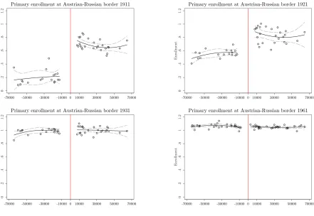
1.5 Discontinuities in primary enrollment at Austrian-Russian border . . . 33

1.6 Discontinuities in literacy at Prussian-Russian border . . . 35

1.7 Discontinuities in literacy at Austrian-Russian border . . . 37

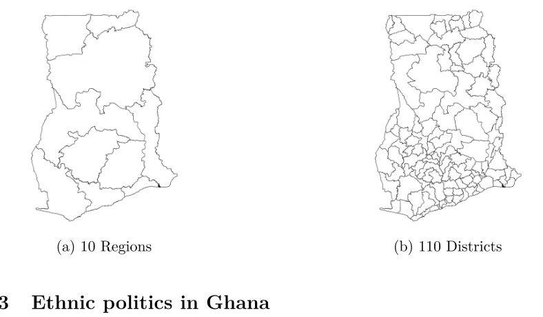
2.1 Administrative divisions of Ghana . . . 54

2.2 Histograms of vote margins in presidential elections 1992-2004 . . . 56

2.3 Margins of victory in presidential elections 1992-2004 . . . 56

2.4 Spatial distribution of vote margins in presidential elections 1992-2004 . . . 57

3.1 Histograms of nighttime lights at two levels of aggregation . . . 83

3.2 Scatter plots in levels at the regional level . . . 84

3.3 Scatter plots in levels at the district level . . . 84

A.1 Discontinuities in geographic characteristics at Austrian-Russian border . . 91

B.1 Ethnic groups of Ghana . . . 100

(8)

List of Tables

1.1 Log population at partition borders in 1810 (One-dimensional RDD) . . . 25

1.2 Log population at partition borders in 1810 (Two-dimensional RDD) . . . 25

1.3 Discontinuities in geographic characteristics . . . 27

1.4 Discontinuities in agriculture . . . 28

1.5 Primary enrollment at Prussian-Russian border 1911-1961 . . . 30

1.6 Primary enrollment at Austrian-Russian border 1911-1961 . . . 32

1.7 Literacy at Prussian-Russian border 1921-1960 . . . 34

1.8 Literacy at Austrian-Russian border 1921-1960 . . . 36

1.9 Robustness of the two-dimensional RDD . . . 38

1.10 Enrollment at Prussian-Russian border 1911-1931, population controls . . 40

1.11 Enrollment at Austrian-Russian border 1911-1931, population controls . . 41

1.12 Literacy at Prussian-Russian Border 1921-1931, population controls . . . . 42

1.13 Literacy at Austrian-Russian border 1921-1931, population controls . . . . 43

1.14 Schools, classes, teachers at partition borders 1911-1961 . . . 45

2.1 Co-ethnicity and economic prosperity 1992-2008 . . . 61

2.2 Co-ethnicity and economic prosperity by governments 1992-2008 . . . 62

2.3 Ewe and Asante districts’ economic prosperity by governments 1992-2008 . 63 2.4 Close elections and economic prosperity 1992-2008 . . . 65

2.5 Close elections, Akan ethnicity and economic prosperity 1992-2008 I . . . . 67

2.6 Close elections, Akan ethnicity and economic prosperity 1992-2008 II . . . 69

2.7 Close elections, other ethnicities and economic prosperity 1992-2008 I . . . 71

2.8 Close elections, other ethnicities and economic prosperity 1992-2008 II . . . 72

3.1 Pooled regressions of nighttime lights and schooling at the regional level . 85 3.2 Pooled regressions of nighttime lights and electrification at the regional level . . . 85

(9)

3.6 Pooled regressions of nighttime lights and electrification at the district level 87

3.7 Panel regressions of nighttime lights and schooling at the district level . . 88

3.8 Panel regressions of nighttime lights and electrification at the district level 88 A.1 Summary statistics at Austrian-Russian border . . . 92

A.2 Summary statistics at Prussian-Russian border . . . 93

A.3 Primary enrollment at Prussian-Russian border 1911-1961 . . . 94

A.4 Primary enrollment at Austrian-Russian border 1911-1961 . . . 95

A.5 Literacy at Prussian-Russian border 1921-1960 . . . 96

A.6 Literacy at Austrian-Russian border 1921-1960 . . . 96

A.7 Enrollment at Prussian-Russian border 1911-1931, population controls . . 97

A.8 Enrollment at Austrian-Russian border 1911-1931, population controls . . 98

A.9 Literacy at Prussian-Russian border 1921-1931, population controls . . . . 99

A.10 Literacy at Austrian-Russian border 1921-1931, population controls . . . . 99

B.1 Summary statistics for the time period 1992-2008 . . . 102

C.1 Summary statistics for the sample at the district level . . . 103

(10)

Preface

Over the recent years, the research domains of development economics and economic his-tory have both witnessed significant augmentations of their empirical toolsets to estimate causal relationships. Differences-in-differences, instrumental variable methods and regres-sion discontinuity designs (RDD) have now become standard techniques as a consequence of what some decided to call “the credibility revolution in empirical economics” (Angrist & Pischke, 2010). At around the same time, both research domains have also benefited from unprecedented expansions of their available data. While economic historians have tapped into the abundant reservoirs of historical maps and statistics, e.g. on education (Becker & Woessmann, 2009; Becker et al., 2014) or income (Piketty, 2003), development economists have been referred to the potential of remote sensing data, in particular night-time lights, by contributions such as Henderson et al. (2012). Unsurprisingly, fruitful overlappings between the two domains have since then followed (e.g. Michalopoulos & Papaioannou, 2013a; Michalopoulos & Papaioannou, 2013b).

The recent advancements in terms of both empirical refinement and data provision mani-fest themselves in the three contributions to development economics and economic history that form the main body of this thesis. Each contribution corresponds to one chapter; all chapters are self-contained and can be read independently from each other.

(11)

Extensive data collection allows me to construct a georeferenced sample on historical school enrollment, school supply and basic human capital covering the partition territo-ries from the times of the empires to the height of communism in Poland. Using the exogeneity of the partition borders for a spatial RDD along the Austrian-Russian and Prussian-Russian borders, I find that the causal effect of the partitions on primary school enrollment is initially large and unfavorable for the partition under Russian rule shortly before the outbreak of World War I (WWI). However, I show that this effect disappears within the following two decades of reconstituted Polish independence. The disappearance is permanent, as there is no evidence for a rebound during the communist era after World War II (WWII). Similarly, the backlog of the Russian partition with regard to literacy declines over time, albeit at a slower rate than schooling, reaching negligible importance in the 1960s. While my investigation suggests that changes in the population composi-tion of Poland were of only minor importance, I provide complementary evidence that the fading imperial legacies on education were accompanied by a substantial expansion of the supply of educational facilities in terms of schools and their endowment.

(12)

agri-cultural suitability (Galor & Özak, 2016) and historical croplands (Ramankutty et al., 1999). Out of the two, the suitability measure is indeed significantly discontinuous at the partition borders. However, I show that the discontinuity completely disappears at the Austrian-Russian border and shrinks to a minuscule size at the Prussian-Russian border once the discontinuous geographical variables are added as controls to the regressions, as suggested by Bukowski (2016). Consequently, all regression results reported in this chapter follow this practice.

To the best of my knowledge, this chapter represents also the first contribution that uti-lizes data that predate the partitions in order to perform a rudimentary check of the absence of pretreatment discontinuities at the borders. So far, the literature has relied on the assessment of historians that the demarcations of the partitions by the three imperial powers were not based on any preexisting demographic, economic or religious conditions, but rather followed military considerations or geographic features such as rivers. I com-plement this assessment with quantitative evidence from a population census conducted in the Duchy of Warsaw in 1810, i.e. before the finalization of the partition borders in 1815. After having georeferenced the data originally published by Grossman (1925), my estimates show no significant discontinuities in (log) population at the future partition borders. While population is arguably a crude correlate of prosperity, its utilization is not uncommon in the literature, which is why I cautiously interpret the absence of population discontinuities in the early 19th century as reassuring for the validity of the spatial RDD at the partition borders.

More generally, this chapter contributes to the literature on the economic history of edu-cation in Europe (Becker & Woessmann, 2009; Becker et al., 2011; Cantoni & Yuchtman, 2013; Squicciarini & Voigtländer, 2015; Dittmar & Meisenzahl, 2016). Further, it appends to the literature on the economic history of Central and Eastern Europe, with Grosfeld et al. (2013) and Markevich et al. (2017) in the context of the Russian Empire, while Becker et al. (2016) focus on legacies of the Austrian-Hungarian Empire.

(13)

ethnic favoritism in Kenya has all but disappeared under democracy. In the broader con-text of sub-Saharan Africa, Franck & Rainer (2012) estimate large and widespread ethnic gains in terms of education and health originating from time periods when an ethnic group has been co-ethnic with its respective country’s leader. On average, these gains remain unaffected by whether the form of government is democratic or autocratic. De Luca et al. (2016) document widespread favoritism in terms of nighttime lights on the level of ethnic homelands. Using a global dataset, they suggest that ethnic favoritism is common across, but not limited to sub-Saharan Africa, with rather negligible dampening effects of the quality of political institutions.

Under which circumstances could ethnic favoritism actually occur in a democratic system of governance? As pointed out by Amodio & Chiovelli (2016), democracy can broaden the scope for strategic interactions between politicians and ethnic leaders. The mixed evidence on the prevalence of ethnic favoritism under democracy suggests that the out-comes of these interactions might be heterogeneous with regard to the extent of ethnic favoritism that they are able to provide (or prevent). From the perspective of economic theories of democracy, the empirical prevalence of ethnic favoritism under democracy can be related to the ‘core’ voter concept of Cox & McCubbins (1986): Political parties differ with regard to their ability to redistribute towards different groups among the electorate, while the groups in turn differ strongly in terms of their ideological party preference. In equilibrium, this results in each party focussing its redistributive efforts on the specific group(s) to which it can redistribute the easiest. Hence, groups are generally not courted by more than one party, making them solid, delimited political blocks which enjoy high patronage as soon as ‘their’ party climbs to power.

(14)

Ashanti empire, exhibit a strong and long-lived ethnic affiliation to the NPP. The NDC, in turn, has strong ties to the Ewe ethnic group, given that Jerry John Rawlings belongs to this group as well.

However, it is questionable whether Ghana’s ethnic setup features the necessary precon-ditions for large-scale redistribution towards the respective president’s co-ethnics because none of the two politically invested groups is actually large enough to secure a majority of the national vote by its own. This suggests that the two political parties rather have to compete for the votes of the more unaffiliated Ghanaian electorate outside of the parties’ ethnic boundaries. This political constellation bears more similarity to the probabilistic or ‘swing’ voting models pioneered by Lindbeck & Weibull (1987) and Dixit & Londregan (1996). The essential prediction of these models is that those groups that contain the highest share of non-partisan, ‘moderate’ voters will be promised the highest share of redistributive transfers by the political parties because the moderates are the most likely to ‘swing’ their votes from one party to the other in return for economic remuneration. Correspondingly, survey evidence in Lindberg & Morrison (2005) and Lindberg (2012) indicates a relatively high and growing share of swing voters among the Ghanaian elec-torate. Evidence by Banful (2011) on the political economy of local budget allocations by the Ghanaian central government further suggests that districts which exhibit tighter vote margins in a presidential election receive higher allocations afterwards. Banful (2011) does not explore any ethnic dimensions of these voting patterns though.

This chapter attempts to broaden the scope for the understanding of ethnic favoritism. It does so by exploiting electoral results and changes of government in Ghana between 1992 and 2008. I first show that the two Ghanaian ethnicities that are co-ethnic with the varying presidents become economically worse off in relative terms soon after the country’s return to democracy. I then test the prediction of the probabilistic voting the-ory that close voting should be associated with economic transfers if there are moderate groups of voters to be swayed. I find that there is indeed a positive association between close voting and economic prosperity, thereby confirming the finding of Banful (2011). However, I further show that this association runs entirely through the homeland of the large, politically unaffiliated ethnic group of the Akan, while it is not detectable with regard to other ethnicities. Taken together, these results suggest that while the eagerness of political parties to form multi-ethnic electoral coalitions has the effect of constraining ethnic favoritism towards the co-ethnics of the respective political leader, the same eager-ness can give rise to ethnic favoritism directed towards groups that signal their readieager-ness to be courted by the political contestants.

(15)

there are no official statistics on economic prosperity at the district level, which is the level of observation in the following, I make use of nighttime lights as a proxy variable. While nighttime lights have already been extensively utilized in the context of ethnic fa-voritism, I reaffirm the usefulness of nighttime lights for detecting patterns of favoritism at the sub-national level.

Nighttime lights as one type of remote sensing data are also central to the third and last contribution of this thesis. Their applications to economics in general and to development economics in particular have been steadily growing over the recent years (Donaldson & Storeygard, 2016; Huang et al., 2014), with the second chapter of this thesis apparently being no deviation from the trend.

Therefore, the third chapter takes a systematic approach to evaluate the applicability and consistency of nighttime lights in the development nexus. Although it is considered good practice to test the applicability of nighttime lights to the respective research context, mostly by correlating them against the variables to be proxied, the settings are so dif-ferent and numerous that they are often not directly comparable with each other. This makes it difficult to derive general conclusions about the applicability and consistency of nighttime lights from them. Therefore, the approach of this chapter attempts to hold as many elements of the empirical framework fixed as possible while switching single param-eters on and off one after another. In order to do so, I construct a spatially harmonized dataset from IPUMS (2017) census extracts. It allows me to examine the behavior of nighttime lights along two important dimensions: Firstly, the level of spatial aggregation can be shifted between the regional and the more disaggregated district level. Secondly, the correlations can be estimated either by pooling all observations or by exploiting the panel structure of the data. While the four resulting combinations are by far not ex-haustive of the potential of nighttime lights, they still provide some clean-cut evidence on the questions whether nighttime lights can be discretionarily utilized in different spatial frameworks without loss of consistency and whether nighttime lights correlate with vari-ables in levels as well as with their changes over time. Thereby, the chapter contributes to the literature that intends to establish nighttime lights as a valid proxy variable in many different applications (Henderson et al., 2012; Chen & Nordhaus, 2011; Chen & Nordhaus, 2015; Hodler & Raschky, 2014; Michalopoulos & Papaioannou, 2013).

(16)

equally strong in terms of statistical significance and also linear in shape.

(17)

Chapter 1 Fading Legacies:

Human Capital in the Aftermath of

the Partitions of Poland

“Dla chcącego nic trudnego.” For the willing, nothing is difficult. (Polish proverb)

1.1 Introduction

The consensus of the empirical literature on economic history is that history matters (see Nunn, 2009, for a review). The persistence of history and thereby the importance of histor-ical legacies have been documented for institutions (Acemoglu et al., 2001; Michalopoulos & Papaioannou, 2013), human capital (Glaeser et al., 2004; Valencia, 2015), and technol-ogy (Comin et al., 2010), to name only a few examples.

Indeed, it would actually be rather surprising if history did not matter: As Wittenberg (2015) points out,any conceivable outcome must necessarily result fromsomeprior causal factor. From this perspective, a legacy from the past is as much a product of history as a non-legacy. Considering, for example, on a large scale the fact that basic education has virtually become universal in all western European nations over the course of the 19th century, it should be evident that history mattered tremendously by turning more than a millennium of persistent human illiteracy into a non-legacy.

(18)

within the boundaries of Poland since 1944.

Figure 1.1: Partition territories within national boundaries of Poland

(a) Partition counties in interwar Poland

(b) Partition counties in Poland since 1944

While Grosfeld & Zhuravskaya (2015) show that the past economic and educational dis-parities cannot be detected along the former partition borders in present-day Poland anymore, I intend to decompress the Polish history that led up to this important result in the spirit of Austin (2008).

Extensive data collection allows me to construct a georeferenced sample on historical school enrollment, school supply and basic human capital covering the partition territo-ries from the times of the empires to the height of communism in Poland. Using the exogeneity of the partition borders for a spatial regression discontinuity design (RDD) along the Austrian-Russian and Prussian-Russian borders, I find that the causal effect of the partitions on primary school enrollment is initially large and unfavorable regarding the partition under Russian rule shortly before the outbreak of World War I (WWI). How-ever, I show that the effect disappears within the following two decades of reconstituted Polish independence. The disappearance is permanent, as there is no evidence for a re-bound during the communist era after World War II (WWII). Similarly, the backlog of the Russian partition with regard to literacy declines over time, albeit at a slower rate than schooling, reaching negligible importance in the 1960s. While my investigation suggests that changes in the population composition of Poland were of only minor importance, I provide complementary evidence that the fading imperial legacies on education were accompanied by a substantial expansion of the supply of educational facilities in terms of schools and their endowment.

(19)

border. Complementary evidence suggests that it was transmitted through positive so-cial norms towards education resulting from the Austrian rule. This hypothesis does not conflict with my results of a rapidly fading legacy, as I focus exclusively on the extensive margin of education, while student performance relates to the intensive margin. The par-ticular setting of the Partitions of Poland is also the topic of Wolf (2005) and Trenkler & Wolf (2005), who study the economic integration of the Polish territories between WWI and WWII. My paper is further closely related to Dupraz (2017) who, while in the context of (post-)colonial Africa, also studies the disappearance of a historical legacy in education along an arbitrarily drawn border.

More generally, this paper contributes to the literature on the economic history of educa-tion in Europe (Becker & Woessmann, 2009; Becker et al., 2011; Cantoni & Yuchtman, 2013; Squicciarini & Voigtländer, 2015; Dittmar & Meisenzahl, 2016). Further, it appends to the literature on the economic history of Central and Eastern Europe, with Grosfeld et al. (2013) and Markevich et al. (2017) in the context of the Russian Empire, while Becker et al. (2016) focus on legacies of the Austrian-Hungarian Empire.

The remainder of the paper is structured as follows: In Section 1.2, I outline the historical context of Poland in terms of population and education over the timespan of my sample. Next, I describe the available data in Section 1.3. Section 1.4 comprises my identification strategy, its assumptions and a discussion whether the latter are likely to hold within the framework of the Partitions of Poland. Section 1.5 presents my main results on the causal effect of the partitions on primary school enrollment and literacy in Poland over the period 1911-1960, followed by a concise series of robustness checks. I discuss the mechanisms behind my findings in Section 1.6. Section 1.7 concludes.

1.2 Historical context

The Partitions of Poland represented one of many drastic watersheds in Polish history. Between 1795 and 1918, Poland did not exist as an independent state, as the three neigh-boring powers of the Polish-Lithuanian Commonwealth, namely Prussia, Austria and Russia, had divided the territory of the large, but weakening Commonwealth among each other. Only at the end of WWI, when the Austrian-Hungarian Empire had fallen apart, the Russian Empire had descended into civil war, and the German Empire had been forced to declare a truce, Polish independence was restored in form of the Second Republic of Poland1_{, reflecting the sustained Polish desire for national unity.}

However, Poland could hardly be called a unified nation in 1918. Its borders in the west

(20)

were still to be finalized by the Treaty of Versailles, while its eastern borders were soon to be redrawn by the outcome of the Polish-Soviet war in 1920. It was also still deeply divided within, as the three empires had not failed to leave their marks on the Polish lands. By the time the borders between them were lifted, the partitions differed substan-tially along several dimensions, both materially and less visibly in terms of culture and institutions. At the brink of their independence, the Poles therefore saw themselves con-fronted with the task of consolidating the three former partitions into one national state. This challenge was particularly pronounced in the realm of education, as the empires had cared to very different extents about setting up an actual educational system: Primary schooling had already been obligatory in Prussia and Austria-Hungary for decades, but it had never even been established in the Russian Empire, creating a large disparity in edu-cational attainment between the populations of the partitions. Consequently, addressing this disparity became the prime goal of educational policy in the following decades. The remarks in this section serve two purposes: First, I characterize the population com-position of Poland from the time of the imperial partitions to the period of communism. I do so for the reason that studying the evolution of Poland’s human capital within the framework of the Polish partitions is negligent without paying attention to the simulta-neous evolution of the population that inhabits the partitions at various points in time. Skilled migration, for example, can have long-term effects (Hornung, 2014); therefore it could obscure or inflate any partition effects on human capital if it occurred only on one side of a partition border. On the top of that, the question of potentially selective migra-tions from one partition into another is particularly relevant for the spatial RDD outlined in Section 1.4.1. In short, the Polish population of the partitions has been spatially per-sistent, making it valid for comparisons along the partition borders as history evolves. However, it has become more homogeneous over time by the expulsion and extinction of ethnic minorities. Second, I sketch the various educational policies that were in place over the course of time.

1.2.1 The imperial period (1795-1918)

1.2.1.1 Population composition

(21)

that are still part of Poland today was in majority Polish at the turn of the 20th cen-tury, with the exception of counties that bordered the remainder of the respective empires where the population was more evenly mixed. The urban areas of the Prussian partition posed another exception; Poznan was the only major city there with a Polish population majority over the German inhabitants. In the Kingdom of Poland, the second-largest population group consisted of Jews, while both Jews and Ukrainians constituted sizable minorities in the part of Galicia that would remain with Poland after WWII.

Despite the pronounced differences between the three partitions, population movements across the partition borders appear to have been a very limited phenomenon. While mi-gration statistics are generally scarce in historical contexts, some publications at least decompose a territory’s population with respect to its various places of birth. For exam-ple, according to the Russian Imperial Census of 1897, only 1.3% of the inhabitants of the Kingdom of Poland were born in a foreign country (Gawryszewski, 2005). Similarly, only 1.2% of the inhabitants of Galicia were foreign-born according to the population census of the Austrian-Hungarian Empire of 1910 (Bureau der K.K. Statistischen Zentralkommis-sion, 1914). This may not surprise given that the partition boundaries represented actual national borders, which typically inhibit mobility much more than e.g. administrative boundaries within the same country. In addition, Davies (2005) suggests that border enforcement was particular harsh on the Russian side.

1.2.1.2 Education during the imperial period

(22)

public funds for education. In contrast, the Galician schools were perceived as a means of preserving and fostering Polish culture and identity; thus the Poles developed a positive association to them.

The Russian Empire, in turn, combined a sparse provision of educational infrastructure with a hostile attitude of the educational system towards the Polish citizens. Russia, in contrast to the German and Austrian empires, did not introduce compulsory school-ing prior to WWI; correspondschool-ingly it also provided few educational facilities. Further, the primary schools in the Russian partition typically comprised only three consecutive classes, compared to the seven and eight classes in Austrian and German primary schools. Education was carried out in Russian language only; thereby creating a similar association of education with oppression and forced assimilation on the side of the Poles as in the German partition.

Some aggregate figures give a descriptive idea of the differences in education across the imperial partitions: The population of the Kingdom of Poland amounted to 12.5 million people in 1910. In the same year, the Kingdom of Galicia and Lodomeria had 8 million inhabitants, while the Grand Duchy of Poznan and the part of West Prussia that was to become part of Poland after WWI counted 3.1 million citizens. However, the Kingdom of Poland provided only 3,352 primary schools for its population by contrast with Galicia’s 5,580 and Prussia’s 4,450. This vast difference in school supply is reflected in the share of primary school students among the total population; this share was only 2.3% in the Kingdom of Poland, while it was 13.5% in Galicia and 19.2% in Prussia. Illiteracy had essentially been eradicated everywhere in the German Empire at the turn of the 20th cen-tury when the share of the illiterate population still averaged 59% in the Polish territories of the Russian Empire in 1897 and 56.6% in Galicia in 1900.2

1.2.2 The interwar period (1918-1939)

The Second Republic of Poland, at its core the composite of the three former partition territories, could be equally characterized as a ethnic, lingual, and multi-religious country. This applied in particular to the eastern territories that Poland had annexed after the Polish-Soviet war (1919-1921), as these so-called borderlands (Polish: Kresy) housed large groups of Belarusians, Ukrainians, Lithuanians, and Jews. However,

these territories did not remain part of Poland after WWII; therefore I exclude them from the following analysis.

The lands of the former Prussian provinces of Posen and West Prussia continued to house

(23)

a German minority of considerable size after the Polish takeover. This was not the case in Galicia, where the Austrian-German presence had historically been much lower. More importantly, the size of the German population group in Poland’s west did not stay constant after WWI. The emigration movement that took hold of the Germans in the former Prussian provinces soon after the latter’s transfer to Poland is the object of study of Blanke (1993). While the Polish constitution of 1921 granted every citizen the right of preserving his nationality and developing his mother-tongue and national character-istics, the auspicious constitutional provisions quickly became subject to interpretations regarding whether they applied to entire minority groups, or just to individuals. For example, German was never recognized as a second official language in the interwar re-public. This created the necessity for German officials and associations to demonstrate their proficiency in Polish in order to keep their positions and accreditations; a necessity that many of them could not meet. Unrest among the German population therefore soon resulted in emigration. How much of the German exodus from the former Prussian par-tition was the result of exaggerated panic among the Germans compared to deliberate emigration for economic reasons or forceful displacement remains a matter of historical debate. Historians also attach a varying degree of reasonable doubt to the unbiasedness of both Prussian and Polish ethnic population statistics. But that emigration took place at a large scale is an undisputed fact (Blanke, 1993): The pre-WWI German population of the Prussian partition and Upper Silesia amounted to approximately 1.1 million. By the end of 1921, about 50% of it had already left Poland. Emigration continued during the subsequent decade in significant numbers: As an orientation, the Polish population census of 1931 reports only about 300,000 native German speakers (and about the same number of Protestants) as remaining in the provinces of Poznan and Pomerania.

(24)

also because of the emigration of the German minority, which had created empty space in both rural and urban areas.

1.2.2.2 Education during the interwar period

The first priority of the Second Republic with regard to education was to establish a network of primary (or ‘common’, Polish: powszechny) education in the former Russian partition where obligatory schooling had not previously existed. Consequently, efforts and resources were concentrated on this purpose. Schooling statistics (MWRiOP, 1927) indeed suggest considerable and rapid improvements in primary schooling in the central provinces that are congruent with the former Kingdom of Poland. For example, the num-ber of pupils in primary school rose from about 370,000 in the school year 1910/11 to about 1,200,000 in 1921/22; thereby more than doubling the gross primary enrollment rate from 19.4% to 48.5% over the same time span.

In terms of aligning the different school systems, the number of years of obligatory school-ing was set to seven nationwide, thereby decreasschool-ing it by one year in the former Prussian partition. Pupils were supposed to start school at the age of seven and hence to complete their primary education at 13. (Krzesniak-Firlej et al., 2014)

(25)

became necessary to replenish it with Polish teachers first before operations could fully resume.

In order to avoid assimilation, the remaining Germans turned to minority schools, to which they were legally entitled. However, a minimum of forty school children within any school district was necessary for maintaining a school; a requirement that became more and more difficult to meet by the shrinking German minority. Together with the closure of all German teacher-training facilities and administrative obstacles, this led to a decline in the number of German-language primary schools in the former Prussian partition from about 1,250 in the school year 1921/22 to about 480 in 1925/26. Hence, a lack of inte-gration of the remaining German minority into the reshuffled Polish school system might have depressed enrollment in western Poland at least during the first years after WWI.

1.2.3 The communist period (1944-1960)

Jumping from the interwar period of independence to the era of communism in Poland requires pointing to the drastic population changes and losses that Poland experienced during and after WWII. About 5.2-5.3 million ethnic Poles and Jews are estimated to have perished between 1939 and 1945 (Eberhardt, 2011), amounting to about 15% of Poland’s pre-WWII population. Further, several million Poles were deported from terri-tories that the German Empire or the Soviet Union had annexed. They were sent into the German-controlled Generalgouvernement, abducted to Germany for forced labor, or kept in remote areas of the Soviet Union.

However, the liberation of the Polish territory from German occupation did not yet end the mass movement of people all across the Polish lands. In the Potsdam Agreement, the victorious Allied powers decided to move Poland’s border westwards. Poland was to cede its eastern territories to the Soviet Union, where they became part of the Lithua-nian, Byelorussian, and Ukrainian Soviet Socialist Republics. As compensation, Poland received the remaining German territories of the Prussian state that were located east of the Oder-Neiße line. Due to their geographic location in the Polish People’s Republic, these territories have been called the Northern and Western Territories (Polish: Ziemie Zachodnie i Pólnocne). In the process of annexing them, their German population was to

(26)

borders.

The population in the three former partitions, which now formed the territorial core of Poland, was apparently much less affected by these drastic migrations, as census data from 1950 shows that, at least at the level of provinces, on average more than 90% of the inhabitants of the former partitions had already lived in the same respective province in 1939 (GUS, 1955). Thus, despite the numerous population transfers during wartime, large-scale populationreplacement was confined to the Northern and Western Territories. The Holocaust and the expulsion of Germans raise the question to what extent these events changed the ethnic and religious composition of Poland’s population. The com-munist period makes it difficult to answer this question because of the official concept of a Polish nation united under socialism. However, it is historically accepted that the population of Poland has been much more ethnically homogeneous since the completion of the major population movements after WWII. For example, Eberhardt (2011) estimates that the share of ethnic Poles within the same pre- and post-WWII territories of Poland already rose from 63.9% in 1939 to 85.7% in 1946. It further rose to 97.8% in 1950 due to the continued expulsion of Germans and the emigration of Jewish Holocaust survivors to Israel.

1.2.3.2 Education during the communist period

Needless to say, the loss of lives during WWII also affected Poland’s stock of human cap-ital; in particular because both Soviet and German occupants specifically targeted the Polish intelligentsia. Eberhardt (2011) cites evidence that about every third Pole with a university education perished during the war. Educational instructors were decimated with a similar bias towards the highly-educated ones: While about 28.5% of the university lecturers died, ‘only’ 5.1% of the primary school teachers perished. Educational infras-tructure was not spared the intense destruction of physical assets during wartime: In the school year 1944/45, the number of public primary schools amounted to only 86.6% of the number of prewar schools within the same territory of Poland. The fall in the number of schools was roughly equally distributed across the country; only the province of Pomera-nia operated less than 70% of its facilities in 1944/45 compared to 1937/38. (MWRiOP, 1946)

(27)

private and religious schools; with the effect of eliminating the latter from the educational sector over the course of the 1950s. After some regulatory turmoil in the early postwar years, the duration of obligatory primary education was set to the prewar level of seven years in 1949. It was extended by one year not until 1961. Educational institutions and curricula were sweepingly harmonized under the socialist command. (Dobosiewicz, 1970)

1.3 Data

1.3.1 Data prior to 1918

The existing literature has to the best of my knowledge not used historical data that predates the partition borders in an attempt to test for the absence of pretreatment dis-continuities. In order to perform a rudimentary test, I rely on population data that have been collected during the short-lived reign of the Duchy of Warsaw in 1810. The Duchy had been constituted by Napoleon I in 1807 and comprised, in addition to the core ter-ritories around Warsaw, most of what became the Prussian partition in 1815 and some parts of the future Austrian partition. While the process of the Partitions of Poland had already begun in 1772, the partition borders were finalized only in 1815. They arguably did not change considerably along the Austrian territory of Galicia, but they bore only lit-tle resemblance to the Prussian-Russian borders drawn before the Napoleonic campaigns. The population data are disaggregated into larger cities, as well as into small settlements. They have been compiled and published by Grossman (1925), who also supplemented them with comparable data on towns and cities in Galicia. Because I do not have a map of the lower-level administrative divisions of the Duchy of Warsaw, I georeference each observation individually and calculate the logarithm of its population as a crude measure of the local prosperity.

(28)

binary indicator for cities in my regression models to capture any potential differential effects of private schooling.

Given that the Prussian and Austrian school statistics do not specify the age of the pupils enrolled in primary school, I rely on gross primary enrollment rates, defined as the share of primary school students among the school-age population, in the following. However, their calculation is complicated by the fact that only the Prussian school census directly provides the number of children at primary school age along with the number of pri-mary school students. Therefore, I complement the data on the number of students in the Austrian and Russian partitions with population statistics. The Austrian-Hungarian Empire conducted a population census in 1910 that provides the corresponding data on the number of children at school age at the county level (Bureau der K.K. Statistischen Zentralkommission, 1914). The Russian Empire, however, conducted a population census only in 1897 (in fact, the first and last census of the Russian empire). While I obtain fig-ures on the county-level population in the Russian partition in 1910 from Polish sources, these figures are not decomposed by age. Falski (1925) provides the county-level share of children at school age among the population in 1897, with school age defined in terms of the laws of interwar Poland, i.e. seven to 13 years. Applying this definition to the Russian partition prior to 1918 is in a sense arbitrary, as there was no legal school age in the Russian Empire. However, from the age statistics in the Russian school census, I calculate that about 95% of the students in primary school in 1911 fell into the age range 7-13. Therefore, assuming that the population share computed by Falski (1925) did not change considerably between 1897 and 1910, I multiply it with the total county population in 1910 to obtain the number of children at school age in 1910 and thereupon the enrollment rate within the Russian partition.

1.3.2 Data on the interwar period

The importance that the Second Polish Republic attributed to education is reflected in both the amount and the depth of data on schooling and educational attainment that has been collected by Polish statistical agencies at that time.

The first complete and disaggregated picture of primary education in independent Poland emerges from a series of publications by the Central Statistical Office (GUS, 1922) that provide data on the school year 1920/21. This series is followed by a census of primary schools collected in the school year 1925/26 (MWRiOP, 1927). Finally, the Central Sta-tistical Office provides an annual series of school statistics starting in the school year 1932/33 (GUS, 1934).

(29)

of educational attainment. The second one is less detailed, but continues the data series on literacy. Consequently, I compute the share of the literate population above primary-school age in both time periods.

The province of Silesia, which consisted of the eastern part of the Prussian province of Upper Silesia, is missing in the census of 1921 because the status of this territory had not been ultimately determined by the time the census was conducted. After its inclusion into Poland, the province further saw numerous changes of administrative boundaries due to its urban character and small territorial units. I therefore exclude Silesia and thereby the only immediate, but relatively short Prussian-Austrian partition border segment from my sample in all time periods.

Similar to before WWI, most of the statistical publications report only the number of stu-dents enrolled in primary school in a given year, without providing information on their age. Consequently, I continue to use gross enrollment rates which I calculate for 1921 and 1931 using the population census information on the number of children at school age within each county. For the school year 1925/26, I compute the average school-age population between 1921 and 1931 using the two census datasets in order to obtain an approximate enrollment rate in 1925/26.

1.3.3 Data on the communist period

Population statistics on educational attainment and literacy are taken from the Polish population census of 1960, same as the number of citizens at primary school age (GUS, 1965). I match these with statistics on the number of primary schools and students of the school year 1960/61 (GUS, 1962). I rely only on this time period because of the extensive educational information of the census, the reform of the school system in 1961 and substantial changes in the system of administrative boundaries soon afterwards.

1.3.4 Georeferenced Polish counties

The spatial RDD necessitates a measure of a county’s distance to the former imperial borders. The Euclidean distance, i.e. the shortest line connecting two points if there were no obstacles, of a county’s centroid to the respective border is a natural candidate. In order to perform the corresponding calculations in ArcGIS, I mainly rely on a map of the Second Republic of Poland (WIG 1934)3 _{for the pre-WWII internal boundaries.}

The borders between regions in the west and the south of the Second Republic coincide with the former partition borders, such that the latter can be easily reconstructed. While

(30)

Poland, on the verge of its regained independence, adopted most of its internal admin-istrative boundaries from the three empires that had previously demarcated the Polish territories, several counties have been merged, split up, or rearranged in the course of the decade from 1921 to 1931. I harmonize the boundaries for the sake of using the same number of counties for each time period by drawing on an online repository of legal acts, including administrative changes, of the Polish parliament (ISAP, 2015) and additional georeferenced maps provided by the Mosaic project (MPIDR and CGG, 2011, 2012a, 2012b).

The county boundaries in 1960, likewise obtained from MPIDR and CGG (2012a) do not bear close resemblance to the pre-WWII boundaries anymore. The former partition borders now cut through a small number of counties, which I therefore exclude from the sample. Keeping the bandwidth constant at 65 km, the sample size is reduced by only one county at the Prussian-Russian border in 1960 compared to the pre-WWII sample. However, it increases by 16 at the Austrian-Russian border due to the creation of new counties. While it would be possible to merge some of the new counties in order to bring the sample size closer to the one available for the earlier years, a larger number of obser-vations in 1960 might actually reduce the risk of incorrectly accepting the null hypothesis of a faded partition effect due to imprecise estimation, which is why I leave the county boundaries unchanged.

The counties along the former partition borders within the changing national borders of Poland that are included in my sample as a result of the bandwidth choice of 65 km are displayed in Figure 1.2.

Figure 1.2: Sample counties within national borders of Poland

(a) Partition borders and sample counties within interwar Poland

(31)

1.4 Identification strategy

1.4.1 Spatial regression discontinuity design (RDD)

The Partitions of Poland provide a promising setting for a spatial RDD that allows esti-mating the causal effect of the partitions on human capital in Poland.

The basic idea behind a RDD is that if individual assignment to treatment is determined by an assignment variable exceeding a threshold and if individuals have imprecise control over the assignment variable, then assignment to treatment is randomized for individuals just below and above the threshold. A well-known example from the literature on the economics of education is that if grant eligibility is tied to student performance in a test, then students are unlikely to have precise control over their test scores such that their exact test score is random within a certain neighborhood. This implies that students who score marginally above or below the grant threshold are randomly assigned to treatment and control. Moreover, they are likely to be similar to each other in terms of both ob-servable and unobob-servable pretreatment characteristics, rendering them valid comparison groups. Indeed, if variation in treatment status is randomized around the threshold, then all characteristics determined prior to the realization of the assignment variable should evolve smoothly around the threshold. (Lee & Lemieux, 2010)

In the spatial context, the assignment variable is typically understood as the distance of a spatial object to a multidimensional discontinuity in space such as a border. The assignment variable exceeding the threshold then translates into crossing this border from one territory into another, with the respective territorial affiliation corresponding to either treatment or control status. Consequently, the causal treatment effect can be identified by comparing observations on both sides of the border, but close to it. However, this requires that the units of observation, for example households or firms, could neither deliberately manipulate the course of the border, nor change their location as response to the border in order to receive (or avoid) treatment. Further, it implies that the border had to be constructed exogenously with regard to the spatial distribution of predetermined vari-ables that influence the outcome of interest. Consequently, these varivari-ables should evolve smoothly around the border (Dell, 2010).

(32)

of the partition borders on education, these borders had to be drawn by the partitioning powers in disregard of local conditions that would influence education. These conditions, whether observable or unobservable, should therefore change smoothly at the borders under investigation. Migrations across partitions, in particular if they occurred due to more promising educational opportunities in the Austrian and Prussian empires, would represent a form of manipulating assignment to treatment.

1.4.2 Econometric specification

The literature that employs spatial RDDs distinguishes a one-dimensional and a two-dimensional parametric approach. In the one-two-dimensional approach, the forcing variable, in my case an observation’s distance to a partition border, enters the regression model linearly. Interacting the distance measure Distancei with an Empirei dummy indicating

the treated partition territory the county is located in (i.e. either Austria or Prussia) further allows the effect of the distance to vary at each side of the border. Adding the county’s longitude Xi, latitude Yi, and a vector of controls Ci results in the following regression model that can be estimated by OLS:

yit=αEmpirei+β1Distancei+β2Empirei⋅Distancei+γ1Xi+γ2Yi+δCi+it (1.1)

The parameter α then identifies the causal effect of either the Austrian or the Prussian empire on the outcome y in period t, depending on the border at which the parameter is estimated. The two-dimensional approach proposed by Dell (2010) is not interested in the direct effect of distance to the border as the forcing variable. Instead, it uses a polynomial of latitude and longitude f(Xi, Yi) in order to flexibly control for a county’s

geographic location along the border:

yit=αEmpirei+f(Xi, Yi) +δCi+it (1.2)

Given that I rely on county-level data in the following, the number of observations within a reasonable distance to the partition borders is relatively small. It precludes the uti-lization of more data-intensive nonparametric methods for estimating the effect of spatial discontinuities.

(33)

under consideration. Grosfeld & Zhuravskaya (2015) and Bukowski (2016) choose nar-rower bandwidths of 60 and 50 km respectively; however, their data are disaggregated to the municipality level, thereby providing more observations. Similarly, the choice of the functional form of the longitude-latitude-polynomial f(Xi, Yi)in the two-dimensional

specification invokes a trade-off: Raising the order of the polynomial increases flexibility, but it also amplifies the threat of overfitting the data. Following the recommendation of Gelman & Imbens (2016), I employ a (relatively low-order) quadratic polynomial of latitude and longitude for Equation 1.2.

1.4.3 Validity of the spatial RDD

In order to provide a simple visual impression, I overlay the internal divisions of the Polish state prior to its partitions with the final partition borders of 1815. Figure 1.3 shows that the regional borders of the Polish-Lithuanian Commonwealth in 1770 (MPIDR and CGG, 2012a) and the partition borders are hardly congruent and in areas where they do overlap, they mostly follow rivers. Further, there is no historic evidence that the local

Figure 1.3: Borders of the Polish-Lithuanian Commonwealth and partition borders

Polish population along the partition borders had any possibility for manipulating their assignment to treatment, i.e. for influencing the decision on which side of an imperial border their municipality or city would be located after 1815. Indeed, the absolutist character of the three empires at the time when they agreed upon the partitions makes it unlikely that their subjects were granted any say in these decisions.

(34)

significant estimate at the Austrian border (column 5) when all observations on both sides of the border are included, the significance vanishes as soon as bandwidths narrower than 100km on each side of the border are chosen. Switching to the two-dimensional specification (Table 1.2) does not yield any significant estimate.

Table 1.1: Log population at partition borders in 1810 (One-dimensional RDD)

(1) (2) (3) (4) (5) (6) (7) (8) Dep. Variable Log Population in 1810

Prussian Side = 1 0.036 -0.126 0.078 -0.017 (0.137) (0.184) (0.234) (0.267)

Austrian Side = 1 0.323** 0.247 0.131 0.077 (0.141) (0.157) (0.184) (0.219) Observations 621 245 165 137 621 251 187 145 R-squared 0.140 0.125 0.136 0.076 0.152 0.163 0.198 0.227 Distance, Distance*Partition Yes Yes Yes Yes Yes Yes Yes Yes Latitude/Longitude, City Yes Yes Yes Yes Yes Yes Yes Yes Bandwidth . 100km 65km 50km . 100km 65km 50km

Notes: One-dimensional RDD. Robust standard errors in parentheses. *** p<0.01, ** p<0.05, * p<0.1

Table 1.2: Log population at partition borders in 1810 (Two-dimensional RDD)

(1) (2) (3) (4) (5) (6) (7) (8) Dep. Variable Log Population in 1810

Prussian Side = 1 -0.088 -0.120 -0.002 -0.064 (0.148) (0.179) (0.220) (0.237)

Austrian Side = 1 0.119 0.251 0.195 0.263 (0.141) (0.155) (0.184) (0.204) Observations 538 245 165 137 470 251 187 145 R-squared 0.128 0.136 0.147 0.077 0.183 0.179 0.217 0.243 2nd order Polynomial, City Yes Yes Yes Yes Yes Yes Yes Yes Bandwidth . 100km 65km 50km . 100km 65km 50km

Notes: Two-dimensional RDD. Robust standard errors in parentheses. *** p<0.01, ** p<0.05, * p<0.1

While I am aware of the simplicity of my pretreatment measure, it gives no evident rea-son to question the smoothness of the population distribution at the designated partition borders before 1815. In addition, the claim of the exogeneity of the partition borders is supported by Grosfeld & Zhuravskaya (2015), who review numerous historical sources that suggest that the partition borders did not reflect preexisting economic, ethnic or religious divisions.

(35)

(36)

Table 1.3: Discontinuities in geographic characteristics

(1) (2) (3) (4) (5) (6) Dep. Variable Altitude (m) Precipitation (mm) Temperature (○C)

Austrian-Russian Border

Panel A: One-Dimensional RDD

Austrian Side = 1 -102.805*** -94.181*** -31.772 -31.391** 0.631*** 0.549*** (34.641) (29.948) (34.414) (13.800) (0.168) (0.164)

Observations 44 44 44 44 44 44

R-squared 0.370 0.647 0.417 0.909 0.403 0.492 Distance, Distance*Austrian Side Yes Yes Yes Yes Yes Yes

Panel B: Two-dimensional RDD

Austrian Side = 1 -117.012*** -110.687*** -48.946*** -46.137*** 0.657*** 0.631*** (29.096) (28.448) (9.216) (8.907) (0.164) (0.164)

R-squared 0.741 0.760 0.960 0.965 0.484 0.498 2nd Order Polynomial Yes Yes Yes Yes Yes Yes

Prussian-Russian Border

Panel C: One-Dimensional RDD

Prussian Side = 1 11.001 1.221 0.021 -2.993 -0.047 -0.051 (16.798) (8.568) (15.112) (8.610) (0.290) (0.063)

R-squared 0.213 0.802 0.003 0.651 0.010 0.950 Distance, Distance*Prussian Side Yes Yes Yes Yes Yes Yes

Panel D: Two-dimensional RDD

Prussian Side = 1 10.694 11.253 -0.737 -0.483 -0.133** -0.136** (9.330) (8.501) (6.940) (6.742) (0.065) (0.060)

R-squared 0.714 0.792 0.664 0.701 0.916 0.933 2nd Order Polynomial Yes Yes Yes Yes Yes Yes

Controls No Yes No Yes No Yes

Notes: One- and two-dimensional RDD. Bandwidth 65 km. Robust standard errors in parentheses. *** p<0.01, ** p<0.05, * p<0.1

(37)

total land cover) over several centuries, from which I select the years 1800 and 1900. Results are presented in Table 1.4. The estimated discontinuity in both average and potential crop yields are large and significant at the Russian-Austrian border in both RDDs, suggesting a substantially higher yield at the Austrian side (columns 1 and 3 in Panel A and B). However, the effect becomes negative and insignificant when altitude, precipitation, and temperature are included as geographic controls (columns 2 and 4).

Table 1.4: Discontinuities in agriculture

(1) (2) (3) (4) (5) (6) (7) (8)

Dep. Variable Average Caloric Yield Optimal Caloric Yield Cropland 1800 Cropland 1900

Austrian-Russian Border

Panel A: One-Dimensional RDD

Austrian Side = 1 186.077** -18.295 407.150* -70.439 -0.017 -0.069 -0.033 -0.101

(91.586) (56.696) (229.682) (154.235) (0.047) (0.045) (0.060) (0.060)

Observations 44 44 44 44 44 44 44 44

R-squared 0.405 0.830 0.446 0.790 0.538 0.770 0.500 0.751

Distance, Distance*Austrian Side Yes Yes Yes Yes Yes Yes Yes Yes

Latitude/Longitude, City Yes Yes Yes Yes Yes Yes Yes Yes

Geo Controls No Yes No Yes No Yes No Yes

Panel B: Two-dimensional RDD

Austrian Side = 1 199.198*** -21.583 498.364*** 60.065 0.015 -0.015 0.014 -0.026

(61.451) (21.751) (127.118) (81.472) (0.032) (0.042) (0.042) (0.056)

Observations 44 44 44 44 44 44 44 44

R-squared 0.663 0.950 0.706 0.949 0.818 0.828 0.791 0.804

2nd Order Polynomial, City Yes Yes Yes Yes Yes Yes Yes Yes

Prussian-Russian Border

Panel C: One-Dimensional RDD

Prussian Side = 1 -80.511* -90.582** -227.352* -214.485** 0.006 0.009 0.007 0.012

(45.155) (36.098) (118.438) (103.037) (0.019) (0.016) (0.025) (0.021)

Observations 54 54 54 54 54 54 54 54

R-squared 0.636 0.745 0.650 0.753 0.417 0.566 0.411 0.562

Distance, Distance*Prussian Side Yes Yes Yes Yes Yes Yes Yes Yes

Latitude/Longitude, City Yes Yes Yes Yes Yes Yes Yes Yes

Panel D: Two-dimensional RDD

Prussian Side = 1 -45.711* -27.849 -197.538** -82.676 -0.020 -0.014 -0.027 -0.019

(23.579) (20.215) (81.034) (61.883) (0.019) (0.019) (0.024) (0.026)

Observations 54 54 54 54 54 54 54 54

R-squared 0.882 0.918 0.801 0.902 0.529 0.579 0.529 0.576

2nd Order Polynomial, City Yes Yes Yes Yes Yes Yes Yes Yes

Notes:One- and two-dimensional RDD. Bandwidth 65 km. Robust standard errors in parentheses.

*** p<0.01, ** p<0.05, * p<0.1

(38)

the estimated discontinuity of 91 amounts to less than five percent of this average. This difference is unlikely to account for the large differences in schooling between the Prus-sian and the RusPrus-sian partition. In addition, both employment in agriculture and school enrollment were more prevalent in the Prussian partition than in the Kingdom of Poland during the imperial era, which does not hint at a relevant trade-off between the two. Furthermore, there are no statistically significant discontinuities in historical cropland at any border neither in 1800 nor 1900 (columns 5-8). Nevertheless, I include all three geographic variables as controls in the following regressions for both borders.

The relevance of population movements as a threat to identification has already been discussed in Section 1.2.1.1: There is no evidence for selective migrations (or large migra-tions of any kind) across the various partimigra-tions borders during the imperial era, implying a very limited potential for treatment status manipulation.

1.5 Results

1.5.1 Main results

Table 1.5 presents estimates of the discontinuity in primary enrollment at the Prussian-Russian partition border over the years 1911 to 1961 using the two-dimensional RDD.4 _In

addition to the estimates of the partition effect, I also report the mean of the dependent variable at the Russian side of the border for each time period in the sample. Keeping the bandwidth fixed at 65 kilometers, primary enrollment is estimated to be more than 80 pp higher in the Prussian partition in 1911/12 when the empires were still existent. Less than ten years later and two years in the reinstated Polish Republic, the difference is roughly cut in half. Both findings are consistent with the descriptives cited in Section 1.2.1.2. The partition effect further falls below 10 pp in 1925/26 and loses significance, while it shows a slight rebound in 1931/32 before it fades entirely in 1960/61. The various controls for longitude/latitude, cities and geography increase the precision of the estimates, but they do not impact their size. Besides the partition effect, the steadily increasing mean of enrollment in the Russian partition over time further suggests that the dwindling partition effect is indeed the result of increasing enrollment in the Russian partition instead of a potential convergence of both partitions to a rather mediocre level of enrollment: In 1931/32, (gross) primary enrollment averages already close to 100 percent in the Russian partition. I visualize the development of the Prussian partition effect across four of the five time periods in Figure 1.4.

(39)

Table 1.5: Primary enrollment at Prussian-Russian border 1911-1961

(1) (2) (3)

Dep. Variable Primary Enrollment 1911 Primary Enrollment 1911 Primary Enrollment 1911 Prussian Side = 1 0.822*** 0.822*** 0.832***

(0.016) (0.016) (0.015)

Observations 54 54 54

R-squared 0.996 0.996 0.997

Mean on Russian Side 0.164 0.164 0.164

(0.042) (0.042) (0.044)

R-squared 0.875 0.888 0.902

Dep. Variable Primary Enrollment 1926 Primary Enrollment 1926 Primary Enrollment 1926 Prussian Side = 1 0.060 0.064* 0.066*

(0.040) (0.033) (0.033)

R-squared 0.185 0.645 0.647

(0.027) (0.026) (0.026)

R-squared 0.410 0.528 0.550

Dep. Variable Primary Enrollment 1961 Primary Enrollment 1961 Primary Enrollment 1961 Prussian Side = 1 -0.027 -0.027 -0.031

(0.026) (0.027) (0.037)

R-squared 0.183 0.187 0.215

Mean on Russian Side 1.081 1.081 1.081 2nd Order Polynomial Yes Yes Yes

City Dummy No Yes Yes

Geographic Controls No No Yes

(40)

Figure 1.4: Discontinuities in primary enrollment at Prussian-Russian border

Y axis: Share of primary enrollment. X axis: Distance to the border in kilometers. Negative distance indicates Russian partition. Bandwidth: 65km.

(41)

Table 1.6: Primary enrollment at Austrian-Russian border 1911-1961

(1) (2) (3)

Dep. Variable Primary Enrollment 1911 Primary Enrollment 1911 Primary Enrollment 1911 Austrian Side = 1 0.495*** 0.499*** 0.400***

(0.032) (0.033) (0.043)

R-squared 0.926 0.927 0.945

Dep. Variable Primary Enrollment 1921 Primary Enrollment 1921 Primary Enrollment 1921 Austrian Side = 1 0.226*** 0.232*** 0.156***

(0.036) (0.037) (0.045)

R-squared 0.835 0.838 0.870

Dep. Variable Primary Enrollment 1926 Primary Enrollment 1926 Primary Enrollment 1926 Austrian Side = 1 0.101** 0.100** 0.028

(0.044) (0.047) (0.050)

R-squared 0.381 0.382 0.428

Dep. Variable Primary Enrollment 1932 Primary Enrollment 1932 Primary Enrollment 1932 Austrian Side = 1 -0.007 0.005 -0.009

(0.020) (0.019) (0.027)

R-squared 0.441 0.653 0.662

Dep. Variable Primary Enrollment 1961 Primary Enrollment 1961 Primary Enrollment 1961 Austrian Side = 1 -0.012 -0.010 -0.002

(0.011) (0.012) (0.014)

R-squared 0.114 0.139 0.192

Mean on Russian Side 1.062 1.062 1.062 2nd Order Polynomial Yes Yes Yes

(42)

Figure 1.5: Discontinuities in primary enrollment at Austrian-Russian border

Y axis: Share of primary enrollment. X axis: Distance to the border in kilometers. Negative distance indicates Russian partition. Bandwidth: 65km.

(43)

Table 1.7: Literacy at Prussian-Russian border 1921-1960

(1) (2) (3)

Dep. Variable Share of Literates 1921 Share of Literates 1921 Share of Literates 1921 Prussian Side = 1 0.246*** 0.245*** 0.244***

(0.015) (0.013) (0.012)

R-squared 0.942 0.960 0.967

Dep. Variable Share of Literates 1931 Share of Literates 1931 Share of Literates 1931 Prussian Side = 1 0.197*** 0.196*** 0.192***

(0.012) (0.010) (0.011)

R-squared 0.954 0.973 0.976

Dep. Variable Share of Literates 1960 Share of Literates 1960 Share of Literates 1960

Prussian Side = 1 0.003 0.003 0.011

(0.010) (0.009) (0.009)

R-squared 0.735 0.787 0.862

2nd Order Polynomial Yes Yes Yes

(44)

Figure 1.6: Discontinuities in literacy at Prussian-Russian border

Y axis: Share of adult literates. X axis: Distance to the border in kilometers. Negative distance indicates Russian partition. Bandwidth: 65km.

Backhaus, Andreas (2018): Essays on development economics and economic history. Dissertation, LMU München: Volkswirtschaftliche Fakultät

Essays on Development Economics

and Economic History

Inaugural-Dissertation

zur Erlangung des Grades

Doctor oeconomiae publicae (Dr. oec. publ.)

an der Ludwig-Maximilians-Universität München

2017

vorgelegt von

Andreas Backhaus

Referent: Prof. Dr. Uwe Sunde

Korreferent: Prof. Dr. Ludger Wößmann

Acknowledgements

Contents

List of Figures

List of Tables

Preface

Chapter 1

Fading Legacies:

Human Capital in the Aftermath of

the Partitions of Poland

1.1

Introduction

1.2

Historical context

1.2.1

The imperial period (1795-1918)

1.2.2

The interwar period (1918-1939)

1.2.3

The communist period (1944-1960)

1.3

Data

1.3.1

Data prior to 1918

1.3.2

Data on the interwar period

1.3.3

Data on the communist period

1.3.4

Georeferenced Polish counties

1.4

Identification strategy

1.4.1

Spatial regression discontinuity design (RDD)

1.4.2

Econometric specification

1.4.3

Validity of the spatial RDD

1.5

Results

1.5.1

Main results