The Application of Predictor Feedback in Designing a Preview Controller for Discrete Time Systems with Input Delay

(1)

Liao, F and Liao, Y and Deng, J (2016) The Application of Predictor Feedback in Designing a Preview

Controller for Discrete-Time Systems with Input Delay. Mathematical Problems in Engineering, 2016.

ISSN 1024-123X DOI: https://doi.org/10.1155/2016/3023915

Link to Leeds Beckett Repository record:

http://eprints.leedsbeckett.ac.uk/3046/

Document Version:

Article

Creative Commons: Attribution 4.0

The aim of the Leeds Beckett Repository is to provide open access to our research, as required by

funder policies and permitted by publishers and copyright law.

The Leeds Beckett repository holds a wide range of publications, each of which has been

checked for copyright and the relevant embargo period has been applied by the Research Services

team.

We operate on a standard take-down policy.

If you are the author or publisher of an output

and you would like it removed from the repository, please

contact us

and we will investigate on a

case-by-case basis.

(2)

Research Article

The Application of Predictor Feedback in Designing a Preview

Controller for Discrete-Time Systems with Input Delay

Fucheng Liao,

1

Yonglong Liao,

1

and Jiamei Deng

2

1_{School of Mathematics and Physics, University of Science and Technology Beijing, Beijing 100083, China} 2_{Leeds Sustainability Institute, Leeds Beckett University, Leeds LS2 9EN, UK}

Correspondence should be addressed to Fucheng Liao; [email protected]

Received 15 April 2016; Revised 19 July 2016; Accepted 25 July 2016

Academic Editor: Jean J. Loiseau

Copyright © 2016 Fucheng Liao et al. This is an open access article distributed under the Creative Commons Attribution License, which permits unrestricted use, distribution, and reproduction in any medium, provided the original work is properly cited.

This paper presents a method for designing a type one servomechanism for a discrete-time linear system with input delay subject to a previewable desired output and a nonmeasurable constant disturbance. The tracking problem of a delay system is transformed into a regulation problem of a delay-free system via constructing an augmented error system and a variable substitution. A controller is obtained with delay compensation and preview compensation based on preview control theory and the predictor method. When the state vector is not directly measurable, a full-dimensional observer is offered. The effectiveness of the design method is demonstrated by numerical simulations.

1. Introduction

Preview control is one of the approaches available for pro-ducing a good performance by utilizing future information of the reference signal in the controller. Lots of work on the preview control problem have already been done. One of the early contributions was delineated in [1], in which a state-feedback controller with preview compensation is derived. Furthermore, Katayama et al. used the linear quadratic integral method to study preview control in both discrete-time and continuous-discrete-time systems [2, 3]. Servomechanisms with integral of tracking error and preview compensation are derived. Liao et al. presented a design method of an optimal preview servomechanism for discrete-time systems in multirate sampled systems [4]. Liao et al. studied the preview control problem of discrete-time descriptor sys-tems and produced a preview controller for the syssys-tems

[5]. Recently, infinite-horizon 𝐻_∞ state-feedback preview

tracking control of retarded state-multiplicative stochastic systems was investigated [6]. In many practical designs, preview control draws considerable favor from engineering researchers, for example, robots walking [7–9], motorcycle performance [10, 11], and protection against earthquakes [12]. During the past several decades, there have been very rich research achievements in the area of control systems

with time delay. An early control method for systems with time delay is the Smith predictor [13], which overcomes the dead time effectively by adding a predictor and a compensator in the controller. Furukawa and Shimemura improved the Smith predictor and offered a new control strategy called “predictive control” [14]. The control module consists of a predictor, an observer, and a controller. Thus, the range of the controller’s application is expanded. Manitius and Olbrot studied the problems of finite spectrum assignment (FSA) of delay systems [15]. The resulting controllers involve integral compensation of the input delay and stabilize the closed-loop systems successfully. The FSA method has been a popular tool in dealing with delay systems. Stable conditions and numerical integral rules were given in [16–18] because the introduction of integral compensation in the controller might lead to closed-loop systems becoming unstable in numerical calculation [19]. L´eonard and Abba studied FSA integral con-trol robustness with respect to prediction time uncertainty for an unstable system [20]. The optimal regulation problem was studied for systems with input delay and designed optimal feedback controllers by using the duality principle and the maximum principle [21–23]. The design process was simplified by introducing a quadratic performance index with corresponding input delay in [24]. A nested predictor was established to effectively compensate for the time delay for

(3)

linear systems with both state and input delays [25, 26]. Robust control and function control strategies were given, respectively, for discrete-time delay systems in [27, 28]. More recently, the optimal control problem was studied for systems with both state and input delays based on the method of letting the preview length go to zero [29]. Optimal tracking controllers for the delay systems are obtained.

For discrete-time linear systems, if the input vector has a time delay, then it is necessary to reconsider the design of the preview controller. The input delay system was transformed into a delay-free system by using the discrete lifting technique in [30, 31]. The researchers then obtained a preview controller based on preview control theory. However, it was pointed out that the discrete lifting technique may lead to “dimension disaster,” especially for systems with large delays [23, 32]. Therefore, this paper further studies the preview control problem of linear systems with input delay. A controller with delay compensation and preview compensation will be developed by using the method of predictor feedback.

This paper is organized as follows. An introduction is given in Section 1. Section 2 is a formulation of the problem and gives some basic assumptions. Section 3 uses the preview control method to construct an augmented error system. Based on Section 3, Section 4 derives a preview controller for the original system. Section 5 constructs a full-dimensional observer. And a brief conclusion is drawn in Section 6.

2. Problem Formulation and Basic

Assumptions

Consider a discrete-time system with input delay as follows:

𝑥 (𝑘 + 1) = 𝐴𝑥 (𝑘) + 𝐵𝑢 (𝑘 − 𝑓) + 𝐸𝑤 (𝑘) ,

𝑦 (𝑘) = 𝐶𝑥 (𝑘) , (1)

where𝑥(𝑘) ∈ 𝑅𝑛is the state vector,𝑢(𝑘) ∈ 𝑅𝑟 is the input

vector,𝑦(𝑘) ∈ 𝑅𝑝is the output vector, and𝑤(𝑘) ∈ 𝑅𝑞is the

nonmeasurable constant disturbance. The positive integer𝑓

represents a constant input delay of the system.𝐴 ∈ 𝑅𝑛×𝑛,

𝐵 ∈ 𝑅𝑛×𝑟_,_{𝐶 ∈ 𝑅}𝑝×𝑛_{, and}_{𝐸 ∈ 𝑅}𝑛×𝑞_{are constant matrices. The}

vectors𝑢(−𝑓), 𝑢(−𝑓 + 1), . . . , 𝑢(0)are initial inputs, and the

vector𝑥(0) = 𝑥₀is the initial state. All the initial vectors are

known.

Let𝑟(𝑘) ∈ 𝑅𝑝be the reference signal.

First, we give the following two basic assumptions:

(A1) Let the pairs (𝐴, 𝐵) be stabilizable, let (𝐶, 𝐴) be

detectable, and let the following conditions hold:

rank[𝐴 𝐵

𝐶 0] = 𝑛 + 𝑝 (full row rank) . (2)

(A2) Let the reference signal𝑟(𝑘)be previewable, and its

preview length is 𝑁_𝑟. Namely, at the present time

𝑘, the present value 𝑟(𝑘) as well as the 𝑁_𝑟 future

values𝑟(𝑘 + 1), . . . , 𝑟(𝑘 + 𝑁_𝑟)is available. The future

values of the reference signal beyond time𝑘 + 𝑁_𝑟are

approximated by𝑟(𝑘+𝑁_𝑟); namely,𝑟(𝑘+𝑙) = 𝑟(𝑘+𝑁_𝑟)

(𝑙 ≥ 𝑁_𝑟+ 1). The reference signal𝑟(𝑘)satisfies

lim

𝑘→∞𝑟 (𝑘) = 𝑟, (3)

where 𝑟is a constant vector. This implies that 𝑟(𝑘)

reaches a steady state.

Furthermore, let𝑒(𝑘)be the error signal defined as the

subtraction of𝑦(𝑘)and𝑟(𝑘); that is,

𝑒 (𝑘) = 𝑦 (𝑘) − 𝑟 (𝑘) . (4)

The purpose of this paper is to design a controller with

preview compensation such that the output 𝑦(𝑘) of the

closed-loop system of (1) tracks the reference signal 𝑟(𝑘)

without any static error in the presence of disturbance𝑤(𝑘);

namely,

lim

𝑘→∞𝑒 (𝑘) = 0. (5)

The optimal control method is applied to achieve the goal. The performance index of (1) can be defined as

𝐽 =∑∞

𝑘=1

[𝑒𝑇_{(𝑘) 𝑄}

𝑒𝑒 (𝑘) + Δ𝑢𝑇(𝑘 − 𝑓) 𝐻Δ𝑢 (𝑘 − 𝑓)] , (6)

where𝑄_𝑒 ∈ 𝑅𝑝×𝑝and𝐻 ∈ 𝑅𝑟×𝑟are positive definite weight

matrices.Δis the first-order backward difference operator;

that is,

Δ𝑢 (𝑘) = 𝑢 (𝑘) − 𝑢 (𝑘 − 1) . (7)

Notice that, as used in [2], the performance index (6) uses

the input vector’s differenceΔ𝑢(𝑘)rather than𝑢(𝑘).

Introduc-ing the input vector’s difference into the performance index can make the closed-loop system contain an integrator, which may help the system to eliminate static error [2, 33].

3. Derivation of the Augmented Error System

The basic method of designing a preview controller for (1) is that an augmented error system is constructed firstly, then a controller is derived for the augmented error system by using optimal preview theory and predictor feedback, and finally the controller for the original system is obtained.

Using Δon both sides of the first equation of (1), the

following will stand:

Δ𝑥 (𝑘 + 1) = 𝐴Δ𝑥 (𝑘) + 𝐵Δ𝑢 (𝑘 − 𝑓) , (8)

where it is obvious that the disturbance vector’s difference

Δ𝑤(𝑘)does not appear because the disturbance is a constant.

UsingΔon𝑒(𝑘 + 1)and noticing𝑒(𝑘 + 1) = 𝐶𝑥(𝑘 + 1) −

𝑟(𝑘 + 1), the following will be obtained:

Δ𝑒 (𝑘 + 1) = 𝐶Δ𝑥 (𝑘 + 1) − Δ𝑟 (𝑘 + 1) . (9)

SinceΔ𝑒(𝑘 + 1) = 𝑒(𝑘 + 1) − 𝑒(𝑘), it can be seen from (8) and

(9) that the error signal satisfies

𝑒 (𝑘 + 1) = 𝑒 (𝑘) + 𝐶𝐴Δ𝑥 (𝑘) + 𝐶𝐵Δ𝑢 (𝑘 − 𝑓)

(4)

Combining (8) and (10) yields

𝑋 (𝑘 + 1) = 𝐴𝑋 (𝑘) + 𝐵Δ𝑢 (𝑘 − 𝑓) + 𝐷Δ𝑟 (𝑘 + 1) ,

𝑒 (𝑘) = 𝐶𝑋 (𝑘) , (11)

where

𝑋 (𝑘) = [ 𝑒 (𝑘)

Δ𝑥 (𝑘)] ,

𝐴 = [𝐼𝑝 𝐶𝐴

0 𝐴] ,

𝐵 = [𝐶𝐵

𝐵] ,

𝐶 = [𝐼𝑝 0] ,

𝐷 = [−𝐼𝑝

0 ] .

(12)

Equation (11) is called the augmented error system of (1).

It is appropriate to take𝑒(𝑘) = 𝐶𝑋(𝑘)as the output of (11),

because the output of (1) is𝑦(𝑘)and the reference signal𝑟(𝑘)

is previewable.

Correspondingly, in terms of the augmented state vector 𝑋(𝑘), the performance index (6) can be expressed as

𝐽 =∑∞

𝑘=1

[𝑋𝑇_{(𝑘) 𝑄𝑋 (𝑘) + Δ𝑢}𝑇_{(𝑘 − 𝑓) 𝐻Δ𝑢 (𝑘 − 𝑓)] ,} ₍₁₃₎

where

𝑄 = [𝑄𝑒 0

0 0] . (14)

If a controller Δ𝑢(𝑘) can be derived such that the

performance index (13) minimum is subject to the dynamic

constraint (11), then it is easy to get lim_𝑘→∞𝑋(𝑘) = 0,

and immediately the conclusion lim_𝑘→∞𝑒(𝑘) = 0 holds.

Furthermore, the input𝑢(𝑘)can be solved fromΔ𝑢(𝑘). And,

thus, the purpose is achieved. This is a standard optimal preview control problem.

4. Main Results and Their Proofs

Let us introduce a new input vector

V(𝑘) = Δ𝑢 (𝑘 − 𝑓) . (15)

Substituting (15) into (11) and (13), respectively, the following stands:

𝑋 (𝑘 + 1) = 𝐴𝑋 (𝑘) + 𝐵V(𝑘) + 𝐷Δ𝑟 (𝑘 + 1) ,

𝑒 (𝑘) = 𝐶𝑋 (𝑘) , (16)

𝐽 =∑∞

𝑘=1

[𝑋𝑇(𝑘) 𝑄𝑋 (𝑘) +V𝑇(𝑘) 𝐻V(𝑘)] . (17)

Obviously, (16) is a delay-free system and the perfor-mance criterion (17) has a normal form. Furthermore, it is

known from (A2) that the reference signal𝑟(𝑘)is previewable

in the sense that the future value Δ𝑟(𝑙) (𝑘 ≤ 𝑙 ≤ 𝑘 +

𝑁_𝑟)is available at each instant of time𝑘. This is a preview

control problem in which the system is described as (16), the

quadratic performance index is described as (17), andΔ𝑟(𝑘)

is previewable. The following theorem will stand based on the results of [2].

Theorem 1. If (A1) and (A2) hold and𝑄_𝑒is positive definite, then the preview controller of (16) that minimizes criterion (17) is given by

V(𝑘) = −𝐺_𝑋𝑋 (𝑘) −∑𝑁𝑟

𝑙=1

𝐺_𝑑(𝑙) Δ𝑟 (𝑘 + 𝑙) , (18)

where

𝐺_𝑋= [𝐻 + 𝐵𝑇𝑃𝐵]−1𝐵𝑇𝑃𝐴,

𝐺_𝑑(1) = − [𝐻 + 𝐵𝑇𝑃𝐵]−1𝐵𝑇𝑃 [𝐼𝑝

0] ,

𝐺_𝑑(𝑙) = [𝐻 + 𝐵𝑇𝑃𝐵]−1𝐵𝑇𝑋 (𝑙 − 1) , 𝑙 = 2, . . . , 𝑁̃ 𝑟,

(19)

where𝑃 ∈ 𝑅(𝑝+𝑛)×(𝑝+𝑛)is the positive semidefinite solution of the algebraic Riccati equation:

𝑃 = 𝐴𝑇𝑃𝐴 − 𝐴𝑇𝑃𝐵 [𝐻 + 𝐵𝑇𝑃𝐵]−1𝐵𝑇𝑃𝐴 + 𝑄. (20)

Furthermore, the matrices𝑋(𝑙) ∈ 𝑅̃ (𝑛+𝑝)×𝑝are given by

̃

𝑋 (1) = −𝐴𝑇_𝑐𝑃 [𝐼𝑝

0] ;

̃

𝑋 (𝑙) = 𝐴𝑇𝑐𝑋 (𝑙 − 1) , 𝑙 = 2, . . . , 𝑁̃ 𝑟,

(21)

where𝐴_𝑐is the closed-loop matrix defined by

𝐴_𝑐 = 𝐴 − 𝐵 [𝐻 + 𝐵𝑇𝑃𝐵]−1𝐵𝑇𝑃𝐴. (22)

Remark 2. The future reference signal valueΔ𝑟(𝑘 + 𝑙) (𝑙 =

1, . . . , 𝑁_𝑟)appearing in∑𝑁𝑟

𝑙=1𝐺𝑑(𝑙)Δ𝑟(𝑘 + 𝑙)acts as a preview

compensation in the controller.

The preview controller for the augmented error system (11) can be derived from Theorem 1 by the following method. Combining (15) and (18), the following equation will be obtained:

Δ𝑢 (𝑘 − 𝑓) = −𝐺_𝑋𝑋 (𝑘) −∑𝑁𝑟

𝑙=1

𝐺_𝑑(𝑙) Δ𝑟 (𝑘 + 𝑙) . (23)

Replacing𝑘 − 𝑓with𝑘leads to

Δ𝑢 (𝑘) = −𝐺𝑋𝑋(𝑘 + 𝑓) −

𝑁𝑟 ∑

𝑙=1

(5)

In (24), the current control inputΔ𝑢(𝑘)uses the future

state vector𝑋(𝑘+𝑓). It is necessary to predict the future state

vector to ensure that the controller is executable. Using the stepwise recurrence technique, we solve the state equation of (11):

𝑋 (𝑘 + 1) = 𝐴𝑋 (𝑘) + 𝐵Δ𝑢 (𝑘 − 𝑓) + 𝐷Δ𝑟 (𝑘 + 1) , (25)

and obtain the future value of the state vector

𝑋 (𝑘 + 𝑓) = 𝐴𝑓𝑋 (𝑘) +𝑓−1∑

𝑙=0

𝐴(𝑓−1−𝑙)𝐵Δ𝑢 (𝑘 + 𝑙 − 𝑓)

+𝑓−1∑

𝑙=0

𝐴(𝑓−1−𝑙)𝐷Δ𝑟 (𝑘 + 1 + 𝑙) .

(26)

The future value𝑋(𝑘 + 𝑓)is predicted by (26). According

to Assumption (A2), for the preview length 𝑁_𝑟 ≥ 𝑓, the

vectorsΔ𝑟(𝑘 + 1 + 𝑙)are available at𝑙 = 0, . . . , 𝑓 − 1; for

the preview length 𝑁_𝑟 < 𝑓, the vectorsΔ𝑟(𝑘 + 1 + 𝑙) are

available at 𝑙 = 0, . . . , 𝑁_𝑟 − 1; andΔ𝑟(𝑘 + 1 + 𝑙) = 0 at

𝑙 = 𝑁𝑟, . . . , 𝑓−1. Obviously, the values in (26) are all available.

Equation (26) indicates that the future state vector𝑋(𝑘+𝑓)is

determined by the current state vector𝑋(𝑘), the past control

inputΔ𝑢(𝑘 + 𝑙 − 𝑓) (𝑙 = 0, . . . , 𝑓 − 1), and the future reference

signal’s differenceΔ𝑟(𝑘+1+𝑙) (𝑙 = 0, . . . , 𝑓−1). The predictor

method we used above is a generalization of the predictor feedback method [14].

Substituting (26) into (24), the feedback control law of the augmented error system (11) can be obtained as follows:

Δ𝑢 (𝑘) = −𝐺𝑋𝐴𝑓𝑋 (𝑘)

− 𝐺_𝑋𝑓−1∑

𝑙=0

𝐴(𝑓−1−𝑙)𝐵Δ𝑢 (𝑘 + 𝑙 − 𝑓)

− 𝐺_𝑋𝑓−1∑

𝑙=0

𝐴(𝑓−1−𝑙)𝐷Δ𝑟 (𝑘 + 1 + 𝑙)

−∑𝑁𝑟

𝑙=1

𝐺_𝑑(𝑙) Δ𝑟 (𝑘 + 𝑓 + 𝑙) .

(27)

Considering the last term of∑𝑁𝑟

𝑙=1𝐺𝑑(𝑙)Δ𝑟(𝑘 + 𝑓 + 𝑙)in (27),

if𝑘 + 𝑓 + 𝑙 > 𝑘 + 𝑁_𝑟, letΔ𝑟(𝑘 + 𝑓 + 𝑙) = 0. It is obvious that

(27) is an executable controller of (11) since all of the parts in (27) are known.

Let us derive a preview controller of (1). First, let

𝐺_𝑋𝐴𝑓= [𝐺_𝑒 𝐺_𝑥] , (28)

where𝐺_𝑒 ∈ 𝑅𝑟×𝑝and𝐺_𝑥 ∈ 𝑅𝑟×𝑛; then, (27) can be rewritten

as

Δ𝑢 (𝑘) = −𝐺𝑒𝑒 (𝑘) − 𝐺𝑥Δ𝑥 (𝑘)

− 𝐺_𝑋𝑓−1∑

𝑙=0

𝐴(𝑓−1−𝑙)𝐵Δ𝑢 (𝑘 + 𝑙 − 𝑓)

− 𝐺_𝑋𝑓−1∑

𝑙=0

𝐴(𝑓−1−𝑙)𝐷Δ𝑟 (𝑘 + 1 + 𝑙)

−∑𝑁𝑟

𝑙=1

𝐺_𝑑(𝑙) Δ𝑟 (𝑘 + 𝑓 + 𝑙) .

(29)

It is assumed that the initial values of system (1) and the

reference signal are zeros; namely, for𝑘 = −𝑓, −𝑓 + 1, . . . , 0,

the vectors𝑥(𝑘) = 0,𝑦(𝑘) = 𝑟(𝑘) = 0, and𝑢(𝑘) = 0. Then, the

following result from (29) will be obtained:

𝑢 (𝑘) = −𝐺𝑒

𝑘

∑

𝑗=1

𝑒 (𝑗) − 𝐺_𝑥𝑥 (𝑘)

− 𝐺_𝑋𝑓−1∑

𝑙=0

𝐴(𝑓−1−𝑙)𝐵𝑢 (𝑘 + 𝑙 − 𝑓)

− 𝐺_𝑋𝑓−1∑

𝑙=0

𝐴(𝑓−1−𝑙)𝐷𝑟 (𝑘 + 1 + 𝑙)

−∑𝑁𝑟

𝑙=1

𝐺_𝑑(𝑙) 𝑟 (𝑘 + 𝑓 + 𝑙) .

(30)

Thus, a preview control theory for system (1) will be obtained as follows.

Theorem 3. Let (A1) and (A2) hold, let𝑄_𝑒be positive definite, and let the performance index be defined as (8). Assume that

𝑥(𝑘) = 0,𝑦(𝑘) = 𝑟(𝑘) = 0, and𝑢(𝑘) = 0for𝑘 = −𝑓, −𝑓 +

1, . . . , 0. Then, the preview controller of (1) is given by

𝑢 (𝑘) = −𝐺𝑒

𝑘

∑

𝑗=1

𝑒 (𝑗) − 𝐺_𝑥𝑥 (𝑘) − 𝑓1(𝑘) − 𝑓2(𝑘) , (31)

where

𝑓₁(𝑘) = 𝐺𝑋

𝑓−1

∑

𝑙=0

𝐴(𝑓−1−𝑙)𝐵𝑢 (𝑘 + 𝑙 − 𝑓) ,

𝑓₂(𝑘) = 𝐺_𝑋𝑓−1∑

𝑙=0

𝐴(𝑓−1−𝑙)𝐷𝑟 (𝑘 + 1 + 𝑙)

+∑𝑁𝑟

𝑙=1

𝐺_𝑑(𝑙) 𝑟 (𝑘 + 𝑓 + 𝑙) ,

(32)

𝐺𝑒and𝐺𝑥are determined by (28), and𝐺𝑋and𝐺𝑑are given

(6)

Remark 4. At each time𝑘, for the general term𝑟(𝑘 + 𝑓 + 𝑙)

in∑𝑁𝑟

𝑙=1𝐺𝑑(𝑙)𝑟(𝑘 + 𝑓 + 𝑙), if𝑓 + 𝑙 ≤ 𝑁𝑟, then the real value of

𝑟(𝑘 + 𝑓 + 𝑙)is taken; if𝑓 + 𝑙 > 𝑁_𝑟, then𝑟(𝑘 + 𝑓 + 𝑙) = 𝑟(𝑘 + 𝑁_𝑟)

is taken. This is determined by Assumption (A2).

Remark 5. It is easy to see that the preview controller (31) is

composed of four terms. The first one−𝐺_𝑒∑𝑘_𝑗=1𝑒(𝑗)is the

accumulation of the tracking error, which ensures that the output of the closed-loop system tracks the reference signal

without static error. The second one −𝐺_𝑥𝑥(𝑘) is the state

feedback. The third one−𝑓₁(𝑘)is the compensation of the

input delay. The last one−𝑓₂(𝑘)is the preview compensation

of the reference signal.

According to the character of the reference signal con-sidered here, the abovementioned design method for the preview controller is applicable to some irregular reference signals which cannot be modeled by the dynamic system’s outputs.

Now, let us apply present theory to an air slider linear motor.

Example 6(see [34]). The dynamic equation of the motor is described as follows:

[ ̇𝑥𝑝(𝑡)

̇𝑥V(𝑡)

] = [ [

0 1

0 −𝐷

𝑀 ] ]

[𝑥𝑝(𝑡)

𝑥_V(𝑡)] + [_[

0

𝐾_𝐹

𝑀 ] ]

𝑢 (𝑡 − 𝜏)

+ [ [

0

−1

𝑀 ] ]

𝑑 (𝑡) ,

(33)

where𝑥_𝑝(𝑡)is place,𝑥_V(𝑡)is velocity,𝑢(𝑡)is current input,𝑑(𝑡)

is constant disturbance signal,𝐷is friction factor,𝑀is the

mass of movable part,𝐾_𝐹is propulsive force coefficient, and

𝜏is input delay. The motor’s parameters are𝐾_𝐹= 2.3 (N/A),

𝑀 = 1.82 (kg), and𝐷 = 3.48 (kg/s), and𝜏could be taken as

0.10 (s),0.20 (s), and0.30 (s), respectively.

Let

𝑥 (𝑡) = [𝑥𝑝(𝑡)

𝑥_V(𝑡)] ; (34)

then, (33) can be rewritten as

̇𝑥 (𝑡) = 𝐴0𝑥 (𝑡) + 𝐵0𝑢 (𝑡 − 𝜏) + 𝐸0𝑤 (𝑡) . (35)

The place of𝑥_𝑝(𝑡)is the output vector, and it can be described

as

𝑦 (𝑡) = 𝐶𝑥 (𝑡) , (36)

where

𝐴₀= [

[ 0 1

0 −_𝑀𝐷]_],

𝐵₀= [

[ 0

𝐾_𝐹

𝑀 ] ] ,

𝐸₀= [

[ 0

−1

𝑀 ] ] ,

𝐶 = [1 0] .

(37)

Taking sampling period 𝑇 = 0.01 (s), a discretization

system is obtained:

𝑥 [(𝑘 + 1) 𝑇] = 𝐴𝑥 (𝑘𝑇) + 𝐵𝑢 [(𝑘 − 𝑓) 𝑇] + 𝐸𝑤 (𝑘𝑇) ,

𝑦 (𝑘𝑇) = 𝐶𝑥 (𝑘𝑇) , (38)

where

𝐴 = [1.0 0.009865

0.0 0.913179] ,

𝐵 = [ 0.0

0.017804] ,

𝐸 = [ 0.0

−0.549451] .

(39)

The delay𝑓is determined by𝜏. According to the value of𝜏,

we have𝑓 = 10,𝑓 = 20, and𝑓 = 30, respectively.

The reference signal 𝑟(𝑡) is given as the following two

types.

(1) Step Signal. Let the reference signal be

𝑟 (𝑡) ={_{

{

0, 𝑡 < 0.2,

1, 𝑡 ≥ 0.2 (40)

which can be discretized into

𝑟 (𝑘𝑇) ={_{

{

0, 𝑘 < 20,

1, 𝑘 ≥ 20. (41)

(2) Fading Signal. Let the reference signal be

𝑟 (𝑡) = _{5𝑡 + 0.90}2 sin(5𝜋 (𝑡 + 0.90)) (42)

which can be discretized into

(7)

Reference signal

t(s)

r

and

y

(m)

y:_{𝜏 = 0.10, lr}_{= 0.30}

y:𝜏 = 0.20, l_r= 0.30

y:𝜏 = 0.30, l_r= 0.30

1.4

1.2

1

0.8

0.6

0.4

0.2

0

[image:7.600.57.286.67.279.2]

0 0.1 0.2 0.3 0.4 0.5 0.6 0.7 0.8

Figure 1: The output responses to the step signal with different delays.

0 0.5 1 1.5 2

−0.3 −0.2 −0.1 0 0.1 0.2 0.3 0.4

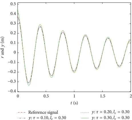
Reference signal

t(s)

r

and

y

(m)

y:𝜏 = 0.10, l_r= 0.30

y:𝜏 = 0.20, l_r= 0.30

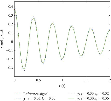
[image:7.600.314.544.71.280.2]

y:𝜏 = 0.30, l_r= 0.30

Figure 2: The output responses to the fading signal with different delays.

Through verification, (𝐴, 𝐵) is stabilizable, (𝐶, 𝐴) is

detectable, and the matrix [𝐴 𝐵_{𝐶 0}] is of full row rank.

Namely, Assumption (A1) is satisfied. We take the weight

matrices𝑄_𝑒= 1.0and𝐻 = 0.005. By Theorem 3, there exists

the preview controller described as (31) for (38).

Let the preview length of the reference signal be 𝑙_𝑟 =

0.30 (s); that is,𝑁_𝑟= 30. The output responses of the

closed-loop system are given as in Figures 1 and 2.

The output responses of the closed-loop system tracking to the step signal are shown in Figure 1 and those to the fading signal are shown in Figure 2. From Figures 1 and 2, it can be seen that the closed-loop’s output can track the reference signal asymptotically with the controller (31). Comparing

Reference signal

t(s)

r

and

y

(m)

y:_{𝜏 = 0.30, lr}_{= 0.30}

y:𝜏 = 0.30, l_r= 0.32

y:𝜏 = 0.30, l_r= 0.35

1.4

1.2

1

0.8

0.6

0.4

0.2

0

[image:7.600.314.544.328.538.2]

0 0.1 0.2 0.3 0.4 0.5 0.6 0.7 0.8

Figure 3: The output responses to the step signal with different preview lengths.

0 0.5 1 1.5 2

−0.3 −0.2 −0.1 0 0.1 0.2 0.3 0.4

Reference signal

t(s)

r

and

y

(m)

y:𝜏 = 0.30, l_r= 0.30

y:𝜏 = 0.30, l_r= 0.32

y:𝜏 = 0.30, l_r= 0.35

Figure 4: The output responses to the fading signal with different preview lengths.

with the output responses with different delays, it can be seen that under the same preview length the tracking performance will get worse when the delay is large.

When the preview length is equal to the input delay, the future value of the reference signal is only used to compensate the delay. In order to get a better performance, let us take a

larger preview length. When the input delay𝜏 = 0.30 (s), the

preview lengths𝑙_𝑟 = 0.30 (s),𝑙_𝑟 = 0.32 (s), and𝑙_𝑟 = 0.35 (s)

are taken; that is𝑁_𝑟 = 30,𝑁_𝑟= 32, and𝑁_𝑟= 35, respectively.

The output responses of the closed-loop system are given as in Figures 3 and 4.

[image:7.600.55.289.329.536.2]

(8)

𝑁_𝑟 = 35, which indicates using the controller with preview compensation can reduce the tracking error and improve the tracking speed efficiently. On the other hand, a proper preview length can give a better response.

5. Observer-Based Controller

If the state vector𝑥(𝑘)cannot be measured directly, then it is

necessary to design an observer to obtain the estimate of the state vector.

Since𝑤(𝑘)is constant but cannot be measured, we take it

as a portion of the desired estimate vector. System (1) can be rewritten as

[𝑥 (𝑘 + 1)

𝑤 (𝑘 + 1)] = [

𝐴 𝐸

0 𝐼_𝑞] [

𝑥 (𝑘)

𝑤 (𝑘)] + [

𝐵

0] 𝑢 (𝑘 − 𝑓) ,

𝑦 (𝑘) = [𝐶 0] [𝑥 (𝑘)

𝑤 (𝑘)] .

(44)

Let ̂𝑥(𝑘) and 𝑤(𝑘)̂ be the estimates of 𝑥(𝑘) and 𝑤(𝑘),

respectively. Let𝑌𝑘−1 be the output values up to the𝑘 − 1

step; namely, 𝑌𝑘−1 = {𝑦(0), 𝑦(1), . . . , 𝑦(𝑘 − 1)}; let ̂𝑈𝑘−𝑓

be the input values up to the𝑘 − 𝑓 step; namely,𝑈̂𝑘−𝑓 =

{̂𝑢(−𝑓), ̂𝑢(−𝑓 + 1), . . . , ̂𝑢(−𝑓 + 𝑘)}. The input vector̂𝑢(𝑖) (𝑖 =

−𝑓, −𝑓 + 1, . . . , −𝑓 + 𝑘)here is obtained by replacing𝑥(𝑘)

bŷ𝑥(𝑘)in (31). Then, based on𝑌𝑘−1and̂𝑈𝑘−𝑓, the full-order

observer for the system of (44) is given by

[̂𝑥 (𝑘 + 1)

̂

𝑤 (𝑘 + 1)] = [

𝐴 𝐸

0 𝐼_𝑞] [

̂𝑥 (𝑘) ̂

𝑤 (𝑘)] + [

𝐵

0] ̂𝑢 (𝑘 − 𝑓)

+ [𝐿𝑥

𝐿𝑤] (𝑦 (𝑘) − ̂𝑦 (𝑘)) ,

̂𝑦 (𝑘) = [𝐶 0] [̂𝑥 (𝑘)

̂

𝑤 (𝑘)] ,

(45)

wherê𝑦(𝑘)is the output of the observer and𝐿_𝑥 ∈ 𝑅𝑛×𝑝and

𝐿𝑤∈ 𝑅𝑞×𝑝are constant gain matrices, which are determined

so that the matrix

𝐴𝐿= [

𝐴 − 𝐿_𝑥𝐶 𝐸

−𝐿_𝑤𝐶 𝐼_𝑞] (46)

is stable.

Lemma 7. Consider delay system (1). If (𝐶, 𝐴)is detectable and the matrix[_{𝐼−𝐴 𝐸}𝐶 0]is of full column rank, then there exist suitable gains𝐿_𝑥∈ 𝑅𝑛×𝑝and𝐿_𝑤 ∈ 𝑅𝑞×𝑝such that (45) serves as a full-order observer of (44).

Proof. According to the conclusions in [2], the pair

([𝐶 0] , [𝐴 𝐸0 𝐼𝑞]) is detectable if and only if (𝐶, 𝐴) is

detectable and the matrix [_{𝐼−𝐴 𝐸}𝐶 0] is of full column rank.

As a consequence, there exist suitable gains𝐿_𝑥 ∈ 𝑅𝑛×𝑝 and

𝐿_𝑤 ∈ 𝑅𝑞×𝑝 _{such that} _𝐴

𝐿 is stable under the conditions in

Lemma 7. That is to say, the characteristic values of𝐴_𝐿are

less than 1. Substituting the second formula of (45) into the first one and collecting the like terms, we get

[̂𝑥 (𝑘 + 1)

̂

𝑤 (𝑘 + 1)] = 𝐴𝐿[

̂𝑥 (𝑘) ̂

𝑤 (𝑘)] + [

𝐵

0] ̂𝑢 (𝑘 − 𝑓)

+ [𝐿𝑥

𝐿_𝑤] 𝑦 (𝑘) .

(47)

Let us define the subtraction of the actual state of (44) and the estimated state of (45)

[̃𝑥 (𝑘)

̃

𝑤 (𝑘)] = [

𝑥 (𝑘)

𝑤 (𝑘)] − [

̂𝑥 (𝑘) ̂

𝑤 (𝑘)] (48)

as estimation error. Notice that the input vector of (44) should

bê𝑢(𝑘−𝑓). Then, it is easy to get the estimation error dynamic

equation as follows:

[̃𝑥 (𝑘 + 1)

̃

𝑤 (𝑘 + 1)] = 𝐴𝐿[

̃𝑥 (𝑘) ̃

𝑤 (𝑘)] . (49)

Since the matrix 𝐴_𝐿 is stable, it follows that [_̃_𝑤(𝑘)̃𝑥(𝑘)]

asymptotically converges to zero; namely,

lim

𝑡→∞[

̃𝑥 (𝑘) ̃

𝑤 (𝑘)] = 0. (50)

Thus, we have

lim

𝑘→∞([

𝑥 (𝑘)

𝑤 (𝑘)] − [

̂𝑥 (𝑘) ̂

𝑤 (𝑘)]) = 0 (51)

which indicates that (45) can serve as a full-order observer of (44). This completes the proof.

From Lemma 7, it is known that̂𝑥(𝑘)and̂𝑤(𝑘)can serve

as the reconstructed states of 𝑥(𝑘) and 𝑤(𝑘), respectively.

Now, a preview control theorem with observer for system (1) is given as follows.

Theorem 8. If (A1) and (A2) hold,𝑄_𝑒is positive definite, the matrix[_{𝐼−𝐴 𝐸}𝐶 0]is of full column rank, and, for𝑘 = −𝑓, −𝑓 +

(9)

Reference signal

t(s)

r

and

y

(m)

y:_{𝜏 = 0.10, lr}_{= 0.30}

y:𝜏 = 0.20, l_r= 0.30

y:𝜏 = 0.30, l_r= 0.30

1.4

1.2

1

0.8

0.6

0.4

0.2

0

[image:9.600.57.286.68.280.2]

0 0.1 0.2 0.3 0.4 0.5 0.6 0.7 0.8

Figure 5: The output responses with state observer to the step signal.

then the closed-loop system of (1) with state observer is given by

𝑥 (𝑘 + 1) = 𝐴𝑥 (𝑘) + 𝐵̂𝑢 (𝑘 − 𝑓) + 𝐸𝑤 (𝑘) , 𝑦 (𝑘) = 𝐶𝑥 (𝑘) ,

𝑒 (𝑘) = 𝑦 (𝑘) − 𝑟 (𝑘) ,

[̂𝑥 (𝑘 + 1)

̂

𝑤 (𝑘 + 1)] = 𝐴𝐿[

̂𝑥 (𝑘) ̂

𝑤 (𝑘)] + [

𝐵

0] ̂𝑢 (𝑘 − 𝑓)

+ [𝐿𝑥

𝐿_𝑤] 𝑦 (𝑘) ,

̂𝑢 (𝑘) = −𝐺_𝑒∑𝑘

𝑗=1

𝑒 (𝑗) − 𝐺_𝑥[𝐼𝑛 0] [_̂̂𝑥 (𝑘)

𝑤 (𝑘)]

− 𝑓₁(𝑘) − 𝑓₂(𝑘) .

(52)

The gain matrices𝐿_𝑥 ∈ 𝑅𝑛×𝑝 and𝐿_𝑤 ∈ 𝑅𝑞×𝑝are constant, which are determined such that the matrix𝐴_𝐿is stable.𝑓₁(𝑘) and𝑓₂(𝑘)have the following forms:

𝑓₁(𝑘) = 𝐺_𝑋𝑓−1∑

𝑙=0

𝐴(𝑓−1−𝑙)𝐵̂𝑢 (𝑘 + 𝑙 − 𝑓) ,

𝑓2(𝑘) = 𝐺𝑋

𝑓−1

∑

𝑙=0

𝐴(𝑓−1−𝑙)𝐷𝑟 (𝑘 + 1 + 𝑙)

+∑𝑁𝑟

𝑙=1

𝐺𝑑(𝑙) 𝑟 (𝑘 + 𝑓 + 𝑙) ,

(53)

0 0.5 1 1.5 2

−0.3

−0.4 −0.2 −0.1 0 0.1 0.2 0.3 0.4 0.5

Reference signal

t(s)

r

and

y

(m)

y:_{𝜏 = 0.10, lr}_{= 0.30}

y:𝜏 = 0.20, l_r= 0.30

y:𝜏 = 0.30, l_r= 0.30

Figure 6: The output responses with state observer to the fading signal.

where𝐺_𝑒and𝐺_𝑥are determined by (28) and𝐺_𝑋and𝐺_𝑑are given by Theorem 1.

Example 9. Consider the control system in Example 6. If the state vector cannot be measured directly, then the technique described in Theorem 8 is used to design a controller for the

plant. The matrix[_{𝐼−𝐴 𝐸}𝐶 0]is of full column rank and therefore

there exists a full-order observer with the form of (45). Let

𝐿_𝑥 = [−288.14 144.77]𝑇 and 𝐿_𝑤 = −22.13 serve as the

observer’s gain matrices. The output responses are described in Figures 5 and 6.

Compared with the responses in Figures 1 and 2, the output responses in Figures 5 and 6 have a larger error in the initial phase; the tracking performances later are almost the same. The simulation results indicate the design methods for the preview controller with full-order observer are effective.

6. Conclusion

In this paper, a class of preview controller problems of discrete-time linear systems with input delay has been solved. A preview controller with delay compensation and preview compensation is derived. The difficulties of input delay are successfully overcome by predictor feedback. A design method of the full state observer is given when the state vector of the system cannot be measured directly. Numerical results show that the present methods are effective.

Further studies are needed on selecting a proper preview length according to the characteristics of the system, which is a complex problem but a significant one.

Competing Interests

[image:9.600.313.544.71.281.2]

(10)

Acknowledgments

The authors would like to thank the National Natural Science Foundation of China for their financial support under Grant no. 61174209.

References

[1] M. Hayase and K. Ichikawa, “Optimal servosystem utilizing future value of desired function,”Transactions of the Society of Instrument and Control Engineers, vol. 5, no. 1, pp. 86–94, 1969. [2] T. Katayama, T. Ohki, T. Inoue, and T. Kato, “Design of an optimal controller for a discrete-time system subject to previewable demand,”International Journal of Control, vol. 41, no. 3, pp. 677–699, 1985.

[3] T. Katayama and T. Hirono, “Design of an optimal servomech-anism with preview action and its dual problem,”International Journal of Control, vol. 45, no. 2, pp. 407–420, 1987.

[4] F. Liao, K. Takaba, T. Katayama, and J. Katsuura, “Design of an optimal preview servomechanism for discrete-time systems in multirate setting,”Dynamics of Continuous, Discrete, and Impulsive Systems Series B: Applications and Algorithms, vol. 10, no. 5, pp. 727–744, 2003.

[5] F. Liao, M. Cao, Z. Hu, and P. An, “Design of an optimal preview controller for linear discrete time causal descriptor systems,”

International Journal of Control, vol. 85, no. 10, pp. 1616–1624, 2012.

[6] E. Gershon and U. Shaked, “𝐻_∞preview tracking control of retarded state-multiplicative stochastic systems,”International Journal of Robust and Nonlinear Control, vol. 24, no. 15, pp. 2119– 2135, 2014.

[7] S. Kajita, F. Kanehiro, K. Kaneko et al., “Biped walking pattern generation by using preview control of zero-moment point,” in

Proceedings of the IEEE International Conference on Robotics and Automation, vol. 2, pp. 1620–1626, Taipei, Taiwan, September 2003.

[8] S. Shimmyo, T. Sato, and K. Ohnishi, “Biped walking pattern generation by using preview control based on three-mass model,”IEEE Transactions on Industrial Electronics, vol. 60, no. 11, pp. 5137–5147, 2013.

[9] S. Czarnetzki, S. Kerner, and O. Urbann, “Observer-based dynamic walking control for biped robots,” Robotics and Autonomous Systems, vol. 57, no. 8, pp. 839–845, 2009. [10] R. S. Sharp, “Optimal preview speed-tracking control for

motorcycles,”Multibody System Dynamics, vol. 18, no. 3, pp. 397–411, 2007.

[11] J. Marzbanrad, Y. Hojjat, H. Zohoor, and S. K. Nikravesh, “Optimal preview control design of an active suspension based on a full car model,”Scientia Iranica, vol. 10, no. 1, pp. 23–36, 2003.

[12] J. Marzbanrad, G. Ahmadi, and R. Jha, “Optimal preview active control of structures during earthquakes,”Engineering Structures, vol. 26, no. 10, pp. 1463–1471, 2004.

[13] O. J. M. Smith, “A controller to overcome dead time,”Journal of Instrument Society of America, vol. 6, no. 2, pp. 28–33, 1959. [14] T. Furukawa and E. Shimemura, “Predictive control for systems

with time delay,”International Journal of Control, vol. 37, no. 2, pp. 399–412, 1983.

[15] A. Z. Manitius and A. W. Olbrot, “Finite spectrum assignment problem for systems with delays,” Institute of Electrical and Electronics Engineers. Transactions on Automatic Control, vol. 24, no. 4, pp. 541–553, 1979.

[16] W. Michiels, S. Mondi´e, D. Roose, and M. Dambrine, “The effect of approximating distributed delay control laws on stability,” inAdvances in Time-Delay Systems, vol. 38 of Lecture Notes in Computer Science and Engineering, pp. 207–222, Springer, Berlin, Germany, 2004.

[17] V. L. Kharitonov, “Predictor-based controls: the implementa-tion problem,”Differential Equations, vol. 51, no. 13, pp. 1675– 1682, 2015.

[18] T. G. Molnar and T. Insperger, “On the robust stabilizability of unstable systems with feedback delay by finite spectrum assignment,”Journal of Vibration and Control, vol. 22, no. 3, pp. 649–661, 2016.

[19] S. Mondi´e and W. Michiels, “Finite spectrum assignment of unstable time-delay systems with a safe implementation,”IEEE Transactions on Automatic Control, vol. 48, no. 12, pp. 2207– 2212, 2003.

[20] F. L´eonard and G. Abba, “Robustness and safe sampling of distributed-delay control laws for unstable delayed systems,”

IEEE Transactions on Automatic Control, vol. 57, no. 6, pp. 1521– 1526, 2012.

[21] M. Basin and J. Rodriguez-Gonzalez, “Optimal control for linear systems with multiple time delays in control input,”IEEE Transactions on Automatic Control, vol. 51, no. 1, pp. 91–97, 2006. [22] M. Basin, J. Rodriguez-Gonzalez, and R. Martinez-Zuniga, “Optimal control for linear systems with time delay in control input,”Journal of the Franklin Institute, vol. 341, no. 3, pp. 267– 278, 2004.

[23] H. Zhang, G. Duan, and L. Xie, “Linear quadratic regulation for linear time-varying systems with multiple input delays,”

Automatica, vol. 42, no. 9, pp. 1465–1476, 2006.

[24] Y. Zhou and Z. Wang, “Optimal feedback control for linear systems with input delays revisited,”Journal of Optimization Theory and Applications, vol. 163, no. 3, pp. 989–1017, 2014. [25] B. Zhou, “Input delay compensation of linear systems with both

state and input delays by nested prediction,”Automatica, vol. 50, no. 5, pp. 1434–1443, 2014.

[26] B. Zhou, “Input delay compensation of linear systems with both state and input delays by adding integrators,”Systems & Control Letters, vol. 82, pp. 51–63, 2015.

[27] S. Xu, J. Lam, B. Zhang, and Y. Zou, “A new result on the delay-dependent stability of discrete systems with time-varying delays,”International Journal of Robust and Nonlinear Control, vol. 24, no. 16, pp. 2512–2521, 2014.

[28] J. Dibl´ık, M. Feˇckan, and M. Posp´ıˇsil, “On the new control functions for linear discrete delay systems,”SIAM Journal on Control and Optimization, vol. 52, no. 3, pp. 1745–1760, 2014. [29] F. Liao and H. Xu, “Application of the preview control method to

the optimal tracking control problem for continuous-time sys-tems with time-delay,”Mathematical Problems in Engineering, vol. 2015, Article ID 423580, 8 pages, 2015.

(11)

[31] M. Cao and F. Liao, “Design of an optimal preview controller for linear discrete-time descriptor systems with state delay,” Inter-national Journal of Systems Science. Principles and Applications of Systems and Integration, vol. 46, no. 5, pp. 932–943, 2015. [32] S.-Y. Han, G.-Y. Tang, and C.-M. Zhang, “Near-optimal

track-ing control for discrete-time systems with delayed input,”

International Journal of Control, Automation and Systems, vol. 8, no. 6, pp. 1330–1335, 2010.

[33] M. Athans, “On the design of P-I-D controllers using optimal linear regulator theory,”Automatica, vol. 7, no. 5, pp. 643–647, 1971.

(12)

Submit your manuscripts at

http://www.hindawi.com

Hindawi Publishing Corporation

http://www.hindawi.com Volume 2014

Mathematics

Journal of

http://www.hindawi.com Volume 2014 Mathematical Problems in Engineering

Hindawi Publishing Corporation http://www.hindawi.com

Differential Equations International Journal of

Volume 2014

http://www.hindawi.com Volume 2014 Hindawi Publishing Corporationhttp://www.hindawi.com Volume 2014

Mathematical PhysicsAdvances in

Complex Analysis

Journal of

Optimization

Journal of

Combinatorics

International Journal of

Journal of

Function Spaces

Abstract and Applied Analysis

International Journal of Mathematics and Mathematical Sciences

Hindawi Publishing Corporation http://www.hindawi.com Volume 2014

The Scientific

World Journal

Discrete Dynamics in Nature and Society

http://www.hindawi.com Volume 2014 Hindawi Publishing Corporation

Discrete Mathematics

Journal of