Subjective well being and engagement in sport: evidence from England

Subjective well­being and engagement in 

sport: evidence from England

Forrest, DK and McHale, IG

Title

Subjective well­being and engagement in sport: evidence from England

Authors

Forrest, DK and McHale, IG

Type

Book Section

URL

This version is available at: http://usir.salford.ac.uk/17951/

Published Date

2011

USIR is a digital collection of the research output of the University of Salford. Where copyright 

permits, full text material held in the repository is made freely available online and can be read, 

downloaded and copied for non­commercial private study or research purposes. Please check the 

manuscript for any further copyright restrictions.

9.

Subjective well- being and

engagement in sport: evidence from

England

David Forrest and Ian McHale

1. INTRODUCTION

One bishop in the nineteenth- century Anglican Church, whenever asked to say Grace before a public dinner, was wont to pronounce: ‘For this food, for our friendship and for all the happiness cricket brings to the World, Thank God.’ Implicitly, the Bishop was hypothesizing that subjective well- being is a function of engagement in sport, and it is this possibility that we address in this chapter.

The issue perhaps has more relevance to public policy now than it did back then in the nineteenth century. In Britain, as in many European countries, the contemporary state takes a major part of the responsibility for providing sports facilities: even where it is private clubs, rather than municipalities, that own and operate the centres and complexes, they are often in receipt of grants from lottery funds or quasi- governmental organizations. This steady stream of revenue underpins access to sport in many areas. But, undoubtedly, it is threatened by the current crisis of government debt. Where public expenditure has to be scaled down, sports budgets represent a ‘soft’ target, partly because it is hard to measure what benefi ts fl ow from the subsidies. It therefore appears to us timely to inves-tigate the question of whether people’s lives are enhanced by participating in sport and whether it is possible to quantify the benefi t.

We take a direct approach. It is argued, for example by Layard (2005), that increasing happiness should be the overriding role of government and, moreover, that this principle provides a practical framework for informing policy decisions because happiness can be measured in a meaningful way by collecting people’s happiness scores. Now routinely included in data- sets from many social surveys worldwide, happiness scores, often on a 1 to 10 scale, are respondents’ answers to a question about how happy their lives are. Patterns of responses to such a question are remarkably similar

across countries (Peiró, 2006) and intuitively appealing (in the sense that things like health and living with a partner are consistently found to be the most important factors contributing to a sense of individual well- being). This has generated increasing confi dence among economists that it is legit-imate to treat happiness scores as direct measures of the elusive concept of utility and, in examining the association between happiness scores and playing sport, we therefore seek to answer the question of whether govern-ment facilitation of participation in sport raises the utility of those who answer the call to play.

Happiness studies is a sub- discipline with a large literature (for a survey from the perspective of economics, see Dolan et al., 2008) but its applica-tion to sport, at least through formal econometric analysis, has been very limited. Kavetos and Szymanski (2010) looked at the impact on happiness not of participation but of national team success. Huang and Humphreys (Chapter 8 in this volume) attempt to quantify the causal impact of exer-cise on self- reported life satisfaction in the USA. Otherwise, there appear to be no prior or contemporaneous studies to report.

2. THE

DATA

Taking Part is an annual survey of the use of leisure time by adults (defi ned as 16 or over) in England. It is commissioned by the UK government’s Department for Culture, Media and Sport in conjunction with stakeholder organizations, such as Sport England. We exploit data from the largest- scale edition of this survey, carried out in the 16 months period up to October, 2006. It collected happiness scores from 27 989 adults in England (not Scotland, Wales or Northern Ireland), along with considerable detail on their leisure activities and a range of information on demographic and socio- economic variables. All interviews were conducted face to face and had a median length in excess of half an hour. Fieldwork was by the British Market Research Bureau. The core sample was deemed representative of the adult population (Williams, 2006) but there was also a booster sample of ethnic minority communities to ensure adequate numbers for meaning-ful analysis of participation in cultural life by race. Data from Taking Part

are lodged in the UK Data Archive (www.data- archive.ac.uk).

answers will be used below not to investigate whether playing sport makes them feel happy on game day (losers of course may not!) but whether there is a more durable eff ect, in short whether it makes them ‘happier people’.

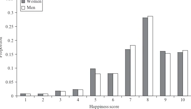
Fortunately for our purpose, the survey asked not only a happiness question (the distribution of the answers to which are illustrated in Figure 9.1) but also whether subjects had participated in active recreational activities in the four weeks preceding the date of the interview. They were shown a list of 60 activities ranging almost from A to Z (American foot-ball to yoga) and were also prompted to mention any others in which they had participated that were not on the list (this uncovered a further eight categories such as frisbee and pilates).

Our focus was to be on sport, so we defi ned our focus variable sports player by reference only to those activities which would conventionally be regarded as sports, as opposed to pastimes or exercise. Of course, a precise defi nition of sport is hard to formulate (see, for example, Farrell and Shields, 2002) and necessarily involves an element of subjectivity. Nevertheless, we decided that partitioning off ‘sports’ from ‘exercise’ was still appropriate. Sport is a distinctive activity that off ers a bundle of characteristics of which exercise is only one: competition (which involves social interaction as well) and skill are other elements which are invariably features of a sport but are not necessarily components of an exercise activ-ity such as jogging. Since they off er diff erent experiences, the relationship between well- being and sport might be misrepresented by examining the

0 0.05 0.1 0.15 0.2 0.25 0.3 0.35

1 2 3 4 5 6 7 8 9 10

Happiness score

Proportion

Women Men

relationship between well- being and an aggregation of sports and exercise activities.

From the list of activities in the survey, many, such as badminton and baseball, cricket and curling, were self- evidently sports. Other pursuits, such as hill trekking and attendance at the gym, we regarded as exercise rather than sport because they lack the element of competition. But a number of cases, including swimming, were ambiguous because they are practised by some participants as keep- fi t and by others competitively. Our criterion with these was to treat as ‘sport’ only those which we judged to be more commonly practised in the context of a contest (the score is kept) than for pure recreation. Accordingly, our fi nal list of ‘sports’ to be used to construct the indicator variable sports player excluded pastimes such as fi shing, skiing, swimming and yachting. On our narrow defi nition, 47.9 per cent of respondents had engaged in sport in the preceding four weeks (a similar order of magnitude to the sports participation rate of 44.5 per cent reported by Farrell and Shields, 2002, from a data- set collected in 1997). Engagement was signifi cantly more common amongst men (54.9 per cent) than among women (42.3 per cent).

3. ARE SPORTS PEOPLE HAPPY PEOPLE?

Mean happiness scores for sports and non- sports players are displayed in Table 9.1. Of course, in calculating means we are implicitly treating the data as cardinal rather than ordinal. But it is not obvious that this is legiti-mate because the gap in happiness implied by a happiness score of 9 as opposed to 8 might not be equivalent to, say, the gap between 5 and 4. On the other hand, Ferrer- i- Carbonell and Frijters (2004) reviewed evidence

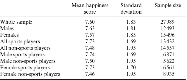
Table 9.1 Sample happiness scores

Mean happiness score

Standard deviation

Sample size

Whole sample 7.60 1.83 27 989

Males 7.63 1.81 12 493

Females 7.57 1.85 15 496

All sports players 7.73 1.69 13 432

All non- sports players 7.48 1.95 14 557

Male sports players 7.74 1.69 6 871

Male non- sports players 7.50 1.95 5 622

Female sports players 7.73 1.70 6 561

consistent with respondents typically answering as if the scale were car-dinal. They attributed this to evolution having given people a common understanding of how numbers are used to convey information concern-ing their feelconcern-ings, such that they treat the choice of numbers ‘much as they interpret weights in the supermarket’. Fortunately, Ferrer- i- Carbonell and Frijters went on to demonstrate that, in practice, it makes little dif-ference which approach is adopted in studying determinants of happiness, since similar patterns emerged from each when they applied them in turn to major happiness data- sets. Here, we treat the data as cardinal but note that no substantive diff erence in qualitative fi ndings emerged when we modelled happiness scores employing methods appropriate to ordinal data. We prefer to present ‘cardinal’ results throughout because of their ease of interpretation.

The raw data in Table 9.1 point to sports people being happier on average than non- sports people. The diff erence of very close to one- quarter of a point is virtually exactly the same whether one considers both genders together or only men or only women. Of incidental interest in Table 9.1 is that the mean and variance of happiness scores of men and women are so close. Here, England may have followed the same path as the USA where the once signifi cant gap in happiness scores (in favour of women) has now entirely disappeared, according to three decades of experience of happiness scores in the General Social Survey (Stevenson and Wolfers, 2008).

That the part of the population playing sport self- reports higher hap-piness than the rest is not in itself very interesting since the diff erence might be due merely to the composition of the two groups. For example, sports people may also be fi nancially better off and in better health on average than non- sports people. What is interesting is to ask whether there is any diff erence in happiness score between otherwise similar people according to whether or not they participate. The answer to this question is most conveniently conveyed through ordinary least squares regression.

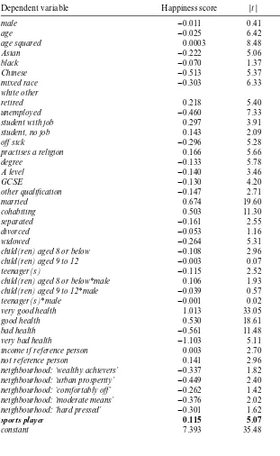
Table 9.2 Ordinary least squares regression results

Dependent variable Happiness score |t |

male −0.011 0.41

age −0.025 6.42

age squared 0.0003 8.48

Asian −0.222 5.06

black −0.070 1.37

Chinese −0.513 5.37

mixed race −0.303 6.33

white other

retired 0.218 5.40

unemployed −0.460 7.33

student with job 0.297 3.91

student, no job 0.143 2.09

off sick −0.296 5.28

practises a religion 0.166 5.66

degree −0.133 5.78

A level −0.140 3.46

GCSE −0.130 4.20

other qualifi cation −0.147 2.71

married 0.674 19.60

cohabiting 0.503 11.30

separated −0.161 2.55

divorced −0.053 1.16

widowed −0.264 5.31

child(ren) aged 8 or below −0.108 2.96

child(ren) aged 9 to 12 −0.003 0.07

teenager(s) −0.115 2.52

child(ren) aged 8 or below*male 0.106 1.93

child(ren) aged 9 to 12*male −0.039 0.57

teenager(s)*male −0.001 0.02

very good health 1.013 33.05

good health 0.530 18.61

bad health −0.561 11.48

very bad health −1.103 5.11

income if reference person 0.003 2.70

not reference person 0.141 2.96

neighbourhood: ‘wealthy achievers’ −0.337 1.82 neighbourhood: ‘urban prosperity’ −0.449 2.40 neighbourhood: ‘comfortably off ’ −0.262 1.42

neighbourhood: ‘moderate means’ −0.376 2.02

neighbourhood: ‘hard pressed’ −0.301 1.62

sports player 0.115 5.07

On the magnitude and signifi cance of most of the control predictor variables, there is a strong consensus across studies irrespective of when and where they were conducted. But there have been mixed fi ndings on whether the subjective wellbeing of adults is aff ected by the presence of children in the household, for example Alesina et al. (2004) found a nega-tive impact. Here we focus on the age rather than the number of children present in the household by including indicator variables to capture the presence or not of one or more children in the young, 9–12 and teenager age groups respectively. Given the possibility that childcare responsibili-ties press more heavily on women, we also include slope dummy variables (for example, young child is multiplied by male)2_{to allow us to show any}

diff erence between men and women in how children infl uence self- reported well- being.

Whether income appears to be an important factor has also varied across studies (for a survey of the relevant literature, see Clark et al., 2008). One of the practical problems in testing is that the same income for an individual could signify poverty (if the level of income is low and the respondent is the breadwinner) or affl uence (if the respondent is a secondary earner and can aff ord to take a part- time or undemanding job). Accordingly, we include income in the model only if the respondent was the ‘household reference person’ (HRP) (for example, if the person was responsible for paying the rent or mortgage, he or she was the HRP; if partners shared the responsibility, the one with higher income was the HRP). We deem the income of non- HRPs as probably not suffi ciently well correlated with family resources to capture living standards and so non- HRPs are represented by setting an appropriate indicator variable to one in their case. It should also be noted that income was collected in the form of bands. We assigned income, which refers to the amount before tax received in the preceding 12 months, as the mid- point of the band. This is unlikely signifi cantly to have distorted the results because the bands were narrow, either £2500 or £5000.3

The survey collected the residential postcode of each respondent and,

Table 9.2 (continued)

Dependent variable Happiness score |t |

Adjusted R- squared 0.139

Number of observations 27 989

employing Geographical Information Systems, this could potentially have given access to a rich set of variables relating to neighbourhood characteristics. But, since each UK postcode refers to a very small area (typically 50 or 100 addresses), these were excluded, for reasons of con-fi dentiality, from the data- set released for use by researchers. However, the public data did include an ACORN (A Classifi cation of Residential Neighbourhoods) code supplied by the commercial service CACI which assigns each postcode in the country to one of a series of neighbourhood descriptors (representing the sort of people who live there) on the basis of very micro- level Census statistics concerning the area in which the postcode is located. This was the source of our set of neighbourhood descriptor indicator variables.

Estimation results displayed in Table 9.2 present familiar patterns. Health is by far the most powerful input in the happiness production func-tion; unemployment is associated with quite severely depressed well- being; it is better to have a partner than to be single; most ethnic minorities are less satisfi ed than white British; well- being is lowest among the middle aged (the turning point in the quadratic relationship between happiness score and age is at age equals 38.05); the religious report themselves happier than others (consistent with Helliwell, 2003); income is a positive factor in determining well- being; and neighbourhood variables play a role (for example, living in an affl uent urban area is a negative predictor of well- being; given that the model holds income constant, this could refl ect either that satisfaction with income is infl uenced by levels of neighbours’ incomes or that high housing costs erode the amount of discretionary spending). There appears to be no diff erence in predicted happiness between those who hold diff erent levels of educational qualifi cation (sug-gesting that benefi ts from extra qualifi cations are only achieved through the income variable) but those with no educational qualifi cation at all are happier (income held constant).

There are novel fi ndings on the eff ect of children. Young children sig-nifi cantly lower happiness scores, though the impact is almost exactly cancelled out by the male slope dummy. Thus we fi nd that the whole cost, in terms of utility, of the burden of looking after young children appears to fall on women. By contrast, both genders seem to suff er equally from a teenager living in the home.

Finally from Table 9.2, the coeffi cient estimate on our focus variable,

4. DOES SPORT MAKE SPORTS PEOPLE HAPPIER

PEOPLE?

Ordinary least squares is an eff ective tool for describing data as it allows us to control for a large number of observed variables. But it cannot allow for the eff ects of non- observed or unobservable variables and that is why, in the present context, our results so far cannot reasonably be interpreted as showing causation running from playing sport to well- being: the results are only descriptive. The problem is that the status of sports player is not dis-tributed randomly within the sample. Rather, sports players self- selected into that group. If they did so on the basis of non- observed or unobserv-able personal characteristics that also had a direct impact on happiness score, then ordinary least squares will yield a biased estimate of the causal

impact of sport on happiness. It will yield an overestimate if the relevant personal characteristics that incline an individual to play sport also tend independently to raise his or her ability to achieve happiness. It will yield an underestimate if the independent eff ect of those characteristics is to tend to lower the ability to achieve happiness.

We had no priors concerning the direction of the bias. Let the decision to play sport depend in part on a set of ‘unknown individual character-istics’. These may be ‘favourable’ in the sense of raising an individual’s capacity to achieve happiness or ‘unfavourable’ in the sense of lowering an individual’s ability to achieve happiness. If positive traits, like being tall or having an extrovert personality, dominate in the infl uence exerted on sports participation by the set of unknown individual characteristics, then persons playing sport will have an atypically high capacity for hap-piness. In ordinary least squares estimation, there will be omitted variable bias such that the infl uence of the non- observed or unobservable indi-vidual characteristics will be captured in an infl ated coeffi cient estimate on sports player. In other words, sports people may be happier because of the sorts of people they are rather than because they play sport. The ordinary least squares coeffi cient estimate on sports player will then be biased upwards.

if they ‘take out’ their aggression on opponents in a setting where this is socially acceptable.

What is suspected here is a type of selection bias that can be addressed with an appropriate statistical model. The two- step treatment eff ects model (for a treatment, see Greene, 2008, pp. 889–90) was developed, within the framework of Heckman, for employment in situations such as we face here. The researcher wishes to estimate the eff ect of treatment (playing sport), represented by a binary variable, on outcome (happiness score). But the decision to undergo treatment is taken by the subject rather than being determined randomly. This raises the possibility of selection bias.

The model proceeds in two stages. The fi rst is a probit to account for the decision whether or not to be treated and the second is the regression of outcome on treatment (and controls). There is selection bias if the errors at stage 1 are correlated with the errors at stage 2. In this event, information extracted at stage 1 is capable of being used at stage 2 to improve explana-tory power and, if it is not, there will be omitted variable bias at stage 2. The treatment eff ects model adds a term, derived from the correlation (if any) between the errors, to capture the infl uence of selectivity and permit the coeffi cient estimate on treatment then to be unbiased.

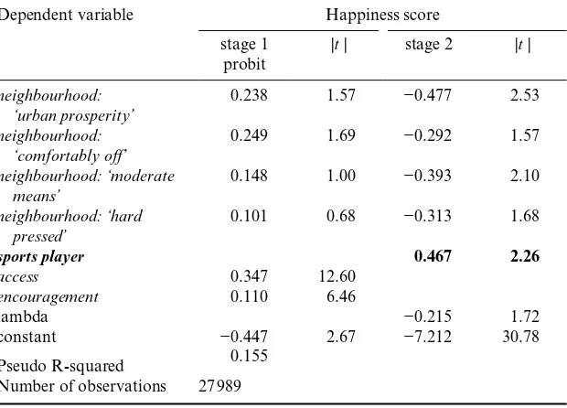
Estimation is enabled to be more precise if it is possible to include exogenous variables at stage 1 which have no direct eff ect on outcome and can therefore be excluded from stage 2. We employed two such variables, each binary. The fi rst is access which is set equal to one for respondents who answered positively to a question on whether sports facilities were available within 20 minutes travelling distance of home (the presence of neighbourhood variables reduces the chance that this will proxy neigh-bourhood quality). The second is encouragement which is set equal to one for respondents who answered positively to a question on whether, as a child, he or she had received parental encouragement to play sport. Unsurprisingly in a small, urbanized country, more than 80 per cent enjoyed access. More than 30 per cent had received encouragement. We judged that neither variable ‘belonged’ in stage 2 because they would be expected to infl uence happiness through the sports player variable rather than directly.

Table 9.3 Treatment eff ects model

Dependent variable Happiness score

stage 1 probit

|t | stage 2 |t |

male 0.316 15.28 −0.048 1.41

age −0.009 2.84 −0.023 5.62

age squared −0.0001 4.18 0.0003 8.59

Asian −0.418 12.11 −0.166 3.02

black −0.343 8.61 −0.023 0.40

Chinese −0.245 2.10 −0.477 3.10

mixed race −0.143 2.33 −0.285 3.38

white other 0.009 0.21

retired 0.134 4.14 0.209 5.11

unemployed 0.100 2.08 −0.471 7.45

student with job 0.108 1.77 0.285 3.72

student, no job 0.155 2.86 0.126 1.81

off sick −0.243 5.25

practises a religion 0.014 0.68 0.165 6.47

degree 0.435 15.98 −0.190 3.91

A level 0.341 13.65 −0.185 4.45

GCSE 0.214 8.88 −0.157 4.51

other qualifi cation 0.064 1.49 −0.153 2.81

married 0.006 0.21 0.671 19.42

cohabiting −0.074 2.15 0.510 11.38

separated −0.029 0.59 −0.158 2.51

divorced 0.123 3.41 −0.068 1.46

widowed 0.033 0.81 −0.273 1.43

child(ren) aged 8 or below −0.087 3.13 −0.097 2.60 child(ren) aged 9 to 12 0.072 2.20 −0.014 0.33

teenager(s) −0.036 1.04 −0.109 2.38

child(ren) aged 8 or below*male

0.026 0.62 0.100 1.81

child(ren) aged 9 to 12*male 0.102 1.90 −0.051 0.73

teenager(s)*male 0.039 0.71 −0.008 0.12

very good health 0.358 15.02 0.969 24.09

good health 0.217 9.74 0.503 15.53

bad health −0.217 5.09 −0.541 10.75

very bad health −0.350 3.79 −1.001 10.55

income if reference person 0.004 4.66 0.002 2.05

not reference person 0.078 3.52 0.131 4.49

neighbourhood: ‘wealthy achievers’

is estimated to raise this by more than 17 percentage points, whereas membership of the Asian community lowers it by very close to 16 percent-age points. Other features of the table include: that males are more likely than females to play sport; that, for a given age and income of course, the unemployed and the retired and students, provided they do not also have a job, are more likely to take part in sport (presumably they are time rich relative to the benchmark); that young children deter parents’ participa-tion but the eff ect is opposite for the 9–12 age group (we speculate that this is the age when parents and children can go to the sports club together); and that cohabitation lowers participation but marriage does not (our interpretation is that most cohabiters are at a stage in their relationship when they still need to be together most of the time). Encouragingly, our two ‘additional’ variables each appear to exert a strong impact on prob-ability of participation with marginal eff ects of more than 13 and more than 4 percentage points for access and encouragement respectively.

In the stage 2 results, the estimated coeffi cient on the selectivity correc-tion term is signifi cant, though weakly so (p 5 .086), and negative. The sign

Table 9.3 (continued)

Dependent variable Happiness score

stage 1 probit

|t | stage 2 |t |

neighbourhood: ‘urban prosperity’

0.238 1.57 −0.477 2.53

neighbourhood: ‘comfortably off ’

0.249 1.69 −0.292 1.57

neighbourhood: ‘moderate means’

0.148 1.00 −0.393 2.10

neighbourhood: ‘hard pressed’

0.101 0.68 −0.313 1.68

sports player 0.467 2.26

access 0.347 12.60

encouragement 0.110 6.46

lambda −0.215 1.72

constant −0.447 2.67 −7.212 30.78

Pseudo R- squared 0.155 Number of observations 27 989

Table 9.4 Reduced- form model

Dependent variable Happiness score |t |

male −0.005 0.20

age −0.025 6.50

age squared 0.0003 8.40

Asian −0.228 5.20

black −0.073 1.42

Chinese −0.503 3.31

mixed race −0.305 3.66

white other −0.206 2.76

retired 0.221 5.48

unemployed −0.454 7.24

student with job 0.294 3.87

student, no job 0.149 2.18

off sick

practises a religion 0.163 6.45

degree −0.128 3.67

A level −0.137 4.26

GCSE −0.129 4.19

other qualifi cation −0.151 2.78

married 0.671 19.50

cohabiting 0.496 11.15

separated −0.163 2.60

divorced −0.050 1.08

widowed −0.262 5.62

child(ren) aged 8 or below −0.011 3.04

child(ren) aged 9 to 12 −0.0009 0.02

teenager(s) −0.113 2.47

child(ren) aged 8 or below*male 0.108 1.97

child(ren) aged 9 to 12*male −0.035 0.51

teenager(s)*male −0.003 0.04

very good health 1.024 33.52

good health 0.534 18.80

bad health −0.562 11.49

very bad health −1.022 10.93

income if reference person 0.003 2.81

not reference person 0.143 5.04

neighbourhood: ‘wealthy achievers’ −0.132 1.79 neighbourhood: ‘urban prosperity’ −0.447 2.39 neighbourhood: ‘comfortably off ’ −0.261 1.41

neighbourhood: ‘moderate means’ −0.378 2.03

neighbourhood: ‘hard pressed’ −0.303 1.63

implies negative correlation between stage 1 and stage 2 errors and so it is suggestive of ordinary least squares giving downwardly biased estimates of the impact of playing sport. It underestimates the impact of sport because it fails to take into account that a disproportionate number of those who are sports players are endowed with unfavourable characteristics from the perspective of wanting to be happy. The point estimate on sports player is 0.467. This represents the causal impact of being a sports player on hap-piness score. It is a large payoff . Though not by any means as important as marriage, the estimated average eff ect of constraining a current player not to take part in sport is almost exactly the same as that from moving a currently employed subject into unemployment. The framework for policy debate in the near future is likely to be on closing sports facilities as a con-tribution to reducing the public sector defi cit. Our results illustrate that participation in sport makes a signifi cant contribution to the well- being of many people and that if closures cause them to give up or play less often, then this would imply a high social cost.

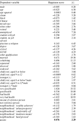
Finally, and similar to Huang and Humphreys (Chapter 8 in this volume), we estimate a reduced form model to check directly the importance of sports facilities. The underlying model is that happiness score depends on the value of sports player (which is endogenous) and the values of control variables. In turn, sports player is a function of the same controls and access

and encouragement. The reduced form equation then has happiness score

depend on all the exogenous variables including access and encouragement. The point estimate on access in Table 9.4 suggests that maintaining the availability of a sports facility to a randomly selected individual raises the expected happiness score by 0.076 points. This could be regarded as a very strong eff ect indeed. For example, if a particular sports centre were the only facility serving the needs of a local population of 1000, the loss in aggregate happiness points from closing it would be roughly equivalent to that from 155 ‘household reference persons’ across the country becoming

Table 9.4 (continued)

encouragement 0.114 2.57

constant 7.354 35.10

Adjusted R- squared 0.141

Number of observations 27 989

unemployed (this takes into account both the direct impact of unem-ployment on happiness score and the eff ect from receiving the sample mean income associated with unemployment rather than the sample mean income associated with employment). As Huang and Humphreys (Chapter 8 in this volume) imply, the loss could be even greater if there is also an eff ect (on well- being) through health variables (which will happen if health suff ers when participation in sport is reduced or terminated). The policy conclusion of our chapter is that sports infrastructure should not lightly be discarded by government.

NOTES

1. The labour force status categories were allocated from answers to questions about whether the interviewee was employed, retired or a student. There was no explicit cat-egory called ‘unemployed’ but we were able to construct our own unemployed variable, set equal to one for those respondents who had not answered ‘employed’ to the main economic status question (they had not done paid work in the preceding seven days) but answered ‘yes’ to a subsequent question about whether they had been looking for work or a place on a training scheme in the preceding four weeks. This left the reference category to include the employed and others, such as homemakers, who were neither students nor retired but who were not seeking a job.

2. Male of course refers to the gender of the respondent, not that of the child.

3. The top band, over £50 000, was unbounded. We gave the respondents in this small cat-egory (3 per cent of the sample) the value of £55 000 but, since this was arbitrary, we also included an indicator variable for this group).

REFERENCES

Alesina, A., Di Tella, R. and MacCulloch, R. (2004), ‘Inequality and happiness: are Europeans and Americans diff erent?’, Journal of Public Economics, 88, 2009–42.

Clark, A.E., Frijters, P. and Shields, M.A. (2008), ‘Relative income, happiness and utility: an explanation for the Easterlin Paradox and other puzzles’, Journal of Economic Literature, 46, 95–144.

Dolan, P., Peasgood, T. and White, M. (2008), ‘Do we really know what makes us happy? A review of the economic literature on the factors associated with sub-jective well- being’, Journal of Economic Psychology, 29, 94–122.

Farrell, L. and Shields, M.A. (2002), ‘Investigating the economic and demo-graphic determinants of sporting participation in England’, Journal of the Royal Statistical Society, Series A, 165, 335–48.

Ferrer- i- Carbonell, A. and Frijters, P. (2004), ‘How important is methodology for the estimates of the determinants of happiness?’, Economic Journal, 114, 641–59.

Helliwell, J.F. (2003), ‘How’s life? Combining individual and national variables to explain subjective well- being’, Economic Modelling, 20, 331–60.

Kavetskos, G. and Szymanski, S. (2010), ‘The impact of major sporting events on happiness’, Journal of Economic Psychology,31 (2), 158–71.

Layard, R. (2005), Happiness: Lessons from a New Science, London: Penguin Books.

Peiró, A. (2006), ‘Happiness, satisfaction and socio- economic conditions: some international evidence’, Journal of Socio- Economics, 35, 348–65.

Stevenson, B. and Wolfers, J. (2008), ‘Happiness inequality in the United States’, Journal of Legal Studies,37,533–79.