210
Design and Simulation of Wideband H-Shape Slot
Loaded Micro-strip Patch Antenna for Wireless
Application
T.Nagarjuna¹, K.Shivaramakrishna², U.Rajini
3,G.Meena
4, K.Ratnaprasad
5, B.Ashok
6¹Assistant Professor, Department of ECE, CMR Technical Campus, JNTU Hyderabad ²˒³,4,5,6
Engineering Project StudentsDepartment of ECE,CMR Technical Campus, JNTU Hyderabad
Abstract- Size reduction of microstrip antenna is very important design consideration. In this paper, design of H-shape microstrip patch antenna with the 2.4GHz frequency for design of antenna. The antenna is simulated using High Frequency Structure Simulator (HFSS). The parameters like VSWR, Return loss, radiation pattern of ordinary microstrip antenna and H-shape Microstrip Patch antenna are designed.
Keywords- Microstrip Patch Antenna, H- Shape Patch Antenna, HFSS, VSWR, Return Loss, Radiation Pattern.
I. INTRODUCTION
Microstrip antenna has many advantages like low cost, less size, light weight, dual and triple frequency operation. Because of less size of microstrip antenna it is used in many wireless applications like satellite communication system, Personal communication system and other wireless applications. In this paper, the main task is to implement more reduced sized microstrip patch antenna without degrading its radiation characteristics, VSWR, Return losses. During period of work first the ordinary microstrip antenna is designed for 2.4GHz then this antenna is simulated by using HFSS software. Then in next step the ordinary patch antenna is modified without changing its length and width and then again this antenna is simulated.[1] Here we want to design the antenna for wireless band so in next step the Length and width of patch is reduced in such a way that antenna is operated in 2.4GHz band of frequency.
[image:1.595.313.532.271.382.2]
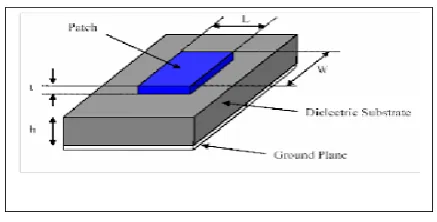
Fig 1: Rectangular micro strip patch antenna
II.ANTENNA GEOMETRY
There are some standard formulae which have to be followed to calculate the length, width, height of the elements used in the antenna design. They are as follows
eff = ⁄ (effective dielectric constant)
Leff = √
(effective length of patch)
( ) ( ) ( )( )
(extended length of patch)
L = Leff - 2
(actual length)
W =
√
211
Lg = 6h + L(Length of ground and substrate)
Wg = 6h + W
(Width of ground and substrate)
Where
h = height of the substrate (1.6mm) f0=operating freq (2 Ghz)
[image:2.595.315.533.154.261.2]r = dielectric constant (4.4) C = speed of light (3* )
Fig 2: Proposed Structure of H-Shaped Rectangular Patch Antenna
III. DESIGN OF H-SHAPE MICROSTRIP PATCH
ANTENNA
The H-shaped microstrip antenna [2] consists of an H shaped patch; supported on a grounded dielectric sheet of thickness h and dielectric constant εr the physical dimensions of the H-shaped microstrip patch antenna are shown in Fig.2. The geometries of the H-shaped slot antenna are shown in figure 2. The antenna is built on a glass epoxy substrate with dielectric constant 4.4 and height h of 1.6 mm. A substrate of low dielectric constant is selected to obtain a compact radiating structure that meets the demanding bandwidth specification. Reducing the size of the antenna is one of the key factors to miniaturize the wireless communication devices. However, reducing the antenna size will usually reduce its impedance bandwidth as well. Therefore designing a small antenna with a wide impedance bandwidth which satisfies future generation wireless application is a challenging work, especially having stable radiation patterns across the operating frequency band [3-4]. In this paper coaxial probe feeding, slot on the patch provide the wide bandwidth and gain enhancement.
IV. SIMULATION AND RESULTS
Fig 3: Graph of Return Loss
[image:2.595.56.280.160.377.2]The simulation is done in HFSS 12.1 (High Frequency Structural Simulator). The simulated result of variation in S11 parameter as a function of frequency for the proposed antenna is shown in fig.3. The noted Return Loss at 1.2000GHz, 3.8000 GHz and 4.000GHz are -6.1527dB,-20.6480dB and –23.7248dB respectively.
Fig 4: Graph for VSWR
[image:2.595.315.533.351.448.2]The VSWR of H-shaped slot loaded microstrip patch antenna has been shown in fig 4. From the plot it has been observed that VSWR at 1.2000,GHz, 3.8000 GHz and 4.000GHz are 9.3685dB,1.6170dB and 1.1330dB respectively.
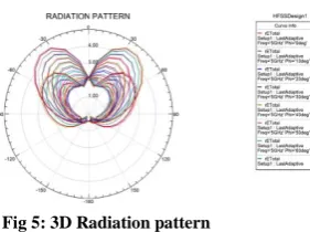
Fig 5: 3D Radiation pattern
[image:2.595.383.524.537.642.2]212
Radiation is the term used to represent the emission or reception of wave front at the antenna, specifying its strength. In any illustration, the sketch drawn to represent the radiation of an antenna is its radiation pattern. One can simply understand the function and directivity of an antenna by having a look at its radiation pattern.Fig 6: Current Distribution
The current distribution plot gives the relationship between the co-polarization (desired) and cross-polarization(undesired) components. Moreover, it gives a clear picture as to the nature of polarization of the fields propagating through the patch antenna. The average current density is shown clearly in figure 6 as different colors on the surface of the antenna which implies that the patch antenna is linearly polarized.
Fig 7: Graph of Smith Chart
The Smith chart is plotted on the complexreflection coefficient plane in two dimensions and is scaled in
normalised impedance (the most common),
normalised admittance or both, using different colours to distinguish between them. These are often known as the Z, Y and YZ Smith charts respectively.[5] Normalised scaling allows the Smith chart to be used for problems involving any characteristic or system impedance which is represented by the center point of the chart. The most
commonly used normalization impedance is 50 ohms.
Once an answer is obtained through the graphical constructions described below, it is straightforward to convert between normalised impedance (or normalised admittance) and the corresponding unnormalized value by multiplying by the characteristic impedance (admittance). Reflection coefficients can be read directly from the chart as they are unitless parameters.
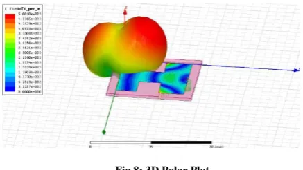
Fig 8: 3D Polar Plot
Typical polar radiation plot.Most antennas show a
[image:3.595.48.265.224.331.2]pattern of "lobes" or maxima of radiation. In a directive antenna, shown here, the largest lobe, in the desired direction of propagation, is called the "main lobe". The other lobes are called "sidelobes" and usually represent radiation in unwanted directions.
Fig 9: Gain 3D polar Plot
In mathematics, the polar coordinate system is a two-dimensional coordinate system in which each point on a plane is determined by a distance from a reference point and an angle from a reference direction.
The reference point (analogous to the origin of a Cartesian coordinate system) is called the pole, and the ray from the pole in the reference direction is the polar axis. The distance from the pole is called the radial coordinate or radius, and the angle is called the angular coordinate, polar angle, or azimuth.[6]
V. CONCLUSION
[image:3.595.67.202.462.553.2]213
VI.ACKNOWLEDGEMENT
we would like to express our gratitude to all those who gave us the support and encouragement to complete the project.
First and foremost, we would thank our project guide Mr. T. NAGARJUNA Sir who supported us throughout and provided the much needed guidance whenever we needed the same. we would like to thank our parents who supported us throughout. who helped us with the final compilation and simulation of my project.
REFERENCES
[1] Constantine A. Balanis “Antenna Theory Analysis and Design” A John Wiley & Sons, Inc., Publication, 2005. pp no.811.
[2] M. Sanad, “Effects of the shorting posts on short microstrip antennas”, Proceeding on IEEE
[3] Mohammad Tariqul Islam, Mohammed Nazbus, Shakib, Norbahiah Misran, Baharudin Yatim, “Analysis of Broadband MicrostripPatch Antenna,” Proc. IEEE, pp. 758-761, 2008.
[4] W. Ren,” Compact dual-band slot antenna for 2.4/5 GHz WLAN applications,” Progress In Electromagnetics Research, B, Vol. 8,319-327, 2008.
[5] Gonzalez, Guillermo (1997) (op. cit);p 97