Thesis by
Nikola Zlatkov Georgiev
In Partial Fulfillment of the Requirements for the Degree of
Doctor of Philosophy
CALIFORNIA INSTITUTE OF TECHNOLOGY Pasadena, California
2019
© 2019
Nikola Zlatkov Georgiev ORCID: 0000-0002-7997-5577
ABSTRACT
The main objective of this thesis is to enable development of high performance
actuation for legged, limbed and mobile robots. Such robots need to support
their own weight, therefore, their actuators need to be light weight, compact, and
efficient. In addition, these actuators need to exhibit significant shock tolerance and backdrivability due to the robots physical contact with the environment. A
dynamics analysis also shows that the actuators’ design may have significant impact
on a robot’s dynamics sensitivity. These consideration motivate improvements in
all actuator design aspects compared to current approaches.
First, the application-specific design of outer rotor motors with concentrated
wind-ings is considered for three main categories: electric vehicles, drones and robotic
joints. It is shown that an intrinsic design trade-off exists between a motor’s cop-per loss, core loss and mass, which allows development of motors with sucop-perior
performance for each application. In particular, it is shown that outstanding torque
density may be reached with high pole count outer rotor motors and the design and
optimization of such motors is outlined in terms of robotic applications. Analytic
motor design scaling modes are also derived to highlight implementation challenges
of high torque motors in robotics.
Next, the design of gearboxes for robotic actuation is discussed. A novel type of
high reduction Bearingless Planetary Gearbox is introduced that allows a large range of reduction ratios to be achieved in a compound planetary stage. In the concept, all
gear components float in an unconstrained manner as the planet carrier is substituted
with a secondary sun gear. This is achieved by introducing an additional kinematic
constraint that allows the planets to be uniform. The advantages of the Bearingless
Planetary Gearbox over current approaches in terms of improved robustness, load
distribution, manufacturability, and assembly are outlined.
Finally, analysis, design, and prototyping of rotary planar springs for rotary series
elastic actuators is described. A model based on curved beam theory that allows rapid iteration and comparison between design parameters of rotary springs is developed.
Mass reduction techniques based on composite arm structures are introduced and
internal arm contact modeling is presented. Motivated by strain energy density
analysis, an optimization based spring design approach is developed that allows
PUBLISHED CONTENT AND CONTRIBUTIONS
[1] Travis Brown et al. “Series Elastic Tether Management for Rappelling Rovers.” In:2018 IEEE/RSJ International Conference on Intelligent Robots and Systems (IROS). IEEE. 2018, pp. 2893–2900. doi:10.1109/IROS. 2018.8594134.
Development of the dual integrated spring design (Sec. 5.2.7) and gear-box with assembled planets (Sec. 4.3.4).
[2] Nikola Georgiev and Joel Burdick. “Optimization-based Design and Analy-sis of Planar Rotary Springs.” In:2018 IEEE/RSJ International Conference on Intelligent Robots and Systems (IROS). IEEE. 2018, pp. 927–934. doi: 10.1109/IROS.2018.8594186.
Optimization-based planar rotary spring design (Sec. 5.4).
[3] Nikola Georgiev and Joel Burdick. “Design and analysis of planar rotary springs.” In: Intelligent Robots and Systems (IROS), 2017 IEEE/RSJ In-ternational Conference on. IEEE. 2017, pp. 4777–4784. doi:10.1109/ IROS.2017.8206352.
Planar rotary spring modeling and analysis (Sec. 5.2).
[4] Nikola Georgiev and Joel Burdick. “Design and analysis of the bearing-less planetary gearbox.” In: Intelligent Robots and Systems (IROS), 2017 IEEE/RSJ International Conference on. IEEE. 2017, pp. 1987–1994. doi: 10.1109/IROS.2017.8206018.
CONTENTS
Abstract . . . iii
Published Content and Contributions . . . iv
Contents . . . v
List of Figures . . . viii
List of Tables . . . xvi
Nomenclature . . . xvii
Chapter I: Introduction . . . 1
1.1 Robotics Actuation . . . 1
1.2 Dual Robotic Actuation . . . 4
1.3 Thesis Structure and Contributions . . . 5
Chapter II: Robot Dynamics Sensitivity . . . 7
2.1 Introduction . . . 7
2.2 Open Chain Manipulator Inverse Dynamics . . . 8
2.3 Limbed and Legged Robot Inverse Dynamics . . . 12
2.4 Robots with Series Elastic Actuators . . . 16
2.5 Example Robot Dynamics Calculations . . . 18
2.5.1 Quadruped robot example . . . 18
2.5.2 RoboSimian . . . 21
2.6 Conclusion . . . 23
Chapter III: Design of Brushless-DC Outer Rotor Motors with Double-layer Concentrated Winding . . . 24
3.1 Introduction . . . 24
3.1.1 Permanent Magnet (PM) Synchronous Motors . . . 25
3.1.2 Contributions and Chapter Structure . . . 27
3.2 Application-specific Motor Design Consideration . . . 28
3.2.1 Motors Designed for EV Applications. . . 29
3.2.2 Motors Designed for Drone Applications. . . 30
3.2.3 Motors Designed for Robotics Applications. . . 31
3.3 Outer Rotor BLDC Motors with Concentrated Winding. . . 33
3.3.1 Outer and Inner Rotor Motors. . . 33
3.3.2 Motor Winding Types. . . 35
3.3.3 Double Layer Concentrated Winding Outer Rotor Motor Modeling . . . 36
3.4 Motor Design Insights, Trade-offs and Guidelines . . . 45
3.4.1 Effect of the Slot Count on the Motor Torque . . . 45
3.4.2 High Pole Count Motors in High Speed Applications . . . . 48
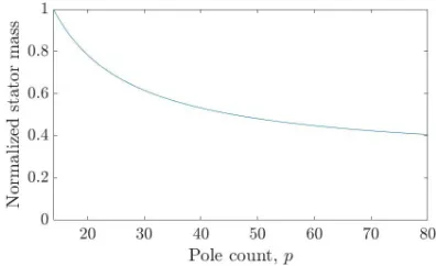
3.4.3 Performance Trade-offs Related to Motor Pole Count . . . . 51
3.4.5 Application Specific Design Guidelines . . . 56
3.4.6 Motor Design Performance Metrics . . . 57
3.5 Verification of the Analytic Model and Design Approach . . . 58
3.5.1 Magnet Width Effect on Motor Torque . . . 58
3.5.2 Slot Factor Analysis Verification . . . 63
3.5.3 Design Trade-offs Verification . . . 66
3.5.4 FEA Comparison of SMPM and IPM Motors . . . 70
3.6 Motor Prototypes . . . 72
3.6.1 EV Prototypes . . . 72
3.6.2 Drone/Robotics Prototype . . . 78
3.6.3 Comparison with Commercially Available Motors . . . 79
3.7 Scaling Modes of PM Motors with Concentrated Windings . . . 81
3.7.1 Motor Rewinding . . . 82
3.7.2 Axial Scaling . . . 83
3.7.3 Radial Scaling . . . 84
3.7.4 Pole Scaling . . . 85
3.7.5 Scaling Laws Discussion . . . 87
3.7.6 Challenges Related to Robotics Application of High Torque Motors. . . 88
3.8 Failure of PM Outer Rotor Motors with Concentrated Windings . . . 89
3.8.1 Mechanical Motor Failure . . . 89
3.8.2 Electrical Motor Failure . . . 90
3.9 Conclusion . . . 91
Chapter IV: Analysis and Design of the Bearingless Planetary Gearbox . . . . 93
4.1 Introduction . . . 93
4.1.1 Speed Reducers Commonly Used in Robotic Applications . 93 4.1.2 Contribution and Chapter Structure . . . 96
4.2 Analysis of The Wolfrom Planetary Gearbox . . . 97
4.2.1 Kinematic Layout . . . 97
4.2.2 Design Requirement for Uniform Planets . . . 99
4.2.3 Strength Analysis . . . 100
4.2.4 Manufacturing and Gearbox Characteristics . . . 102
4.2.5 Application in the Gear Bearing Drive . . . 103
4.2.6 Modifications of the Wolfrom Gearbox . . . 104
4.3 Bearingless Planetary Gearbox . . . 107
4.3.1 Kinematic Layout of the Bearingless Planetary Gearbox . . . 107
4.3.2 Bearingless Planetary Gearbox Strength Analysis . . . 110
4.3.3 Removal of the Planet Assembly Features . . . 118
4.3.4 Bearingless Planetary Gearbox Designs With Assembled Planets . . . 119
4.4 Conclusion . . . 124
Chapter V: Analysis and Design of Planar Rotary Springs . . . 125
5.1 Introduction . . . 125
5.1.1 Previous SEA Rotary Spring Designs . . . 125
5.2 Planar Rotary Spring Modeling . . . 129
5.2.1 Spring Structure . . . 129
5.2.2 Spring Mathematical Model . . . 129
5.2.3 Out-of Plane Buckling . . . 134
5.2.4 Mass Reduction Techniques . . . 135
5.2.5 Archimedean Spiral Arm Spring Designs . . . 137
5.2.6 AR500 Steel Spring Prototype . . . 139
5.2.7 3D-printed Titanium Spring Prototype . . . 147
5.3 Modeling, Simulation and Analysis of Spring Arm Contacts . . . 149
5.3.1 Arm Contact Model . . . 149
5.3.2 Planar Rotary Spring Analysis with Possible Arm Contacts . 151 5.4 Optimization-based Design of Planar Rotary Springs . . . 155
5.4.1 Motivation . . . 155
5.4.2 Optimization-based Design Algorithm . . . 161
5.4.3 7075 Aluminum Spring Prototype . . . 165
5.5 Conclusion . . . 173
Chapter VI: Actuator Prototypes . . . 174
6.1 Chapter Structure and Contributions . . . 174
6.2 Low Reduction Actuator Prototype . . . 175
6.3 Bearingless Series Elastic Actuator . . . 178
6.4 Series Elastic Actuator of Axel Tether Management System . . . 180
Chapter VII: Conclusion and Future Work . . . 182
LIST OF FIGURES
Number Page
1.1 Examples of prismatic [8] ©2014 IEEE and rotary [17] ©2015 IEEE
series elastic actuator designs. . . 2
1.2 Robosimina: NASA Jet Prop. Lab. entry to DRC [33] ©2015 Wiley. 3
2.1 A two-link robot arm driven by gearmotors [37] ©2008 Springer. . . 8
2.2 Open chain manipulator structure. . . 8
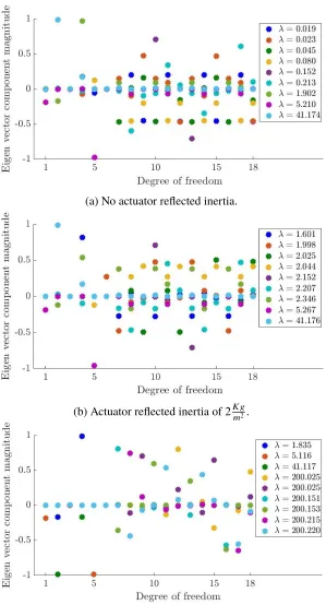
2.3 Quadruped robot model. . . 18
2.4 Representative eigenvectors of the generalized mass matrix of the quadruped robot model of Fig. 2.3 for different values of the actuator
reflected inertia. The corresponding eigenvalues are in the range
from the smallest to the maximum. All actuators are assumed identical. 19
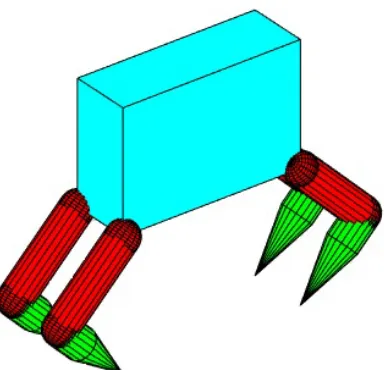
2.5 RoboSimian locomotion stance model. . . 21
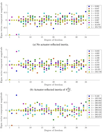
2.6 Representative eigenvectors of Robosimian’s model generalized mass
matrix for different values of the actuator reflected inertia. The
corresponding eigenvalues are in the range from the smallest to the
maximum. All actuators are assumed identical. . . 22
3.1 Motor losses in terms of load and speed. . . 28 3.2 Operating duty cycle of motors depending on the application. . . 28
3.3 High efficiency permanent magnet motors by T-motor used for high
power, heavy lifting quadrotors and airplane drones [79]. . . 30
3.4 Structure of surface mounted permanent magnet inner and outer rotor
motors [81]. The permanent magnets are coloured in red. Left:
inner rotor motor. Right: outer rotor motor (outrunner). The stator
is constructed by teeth and slots (between the teeth) that contain the
winding conductors. See also Fig. 3.6. . . 34
3.5 Stator of distributed winding frameless motor [30] ©2015 IEEE. . . . 35 3.6 Structure of a permanent magnet outer rotor motor with concentrated
windings. The stator slots contain the phase winding conductors. . . 37
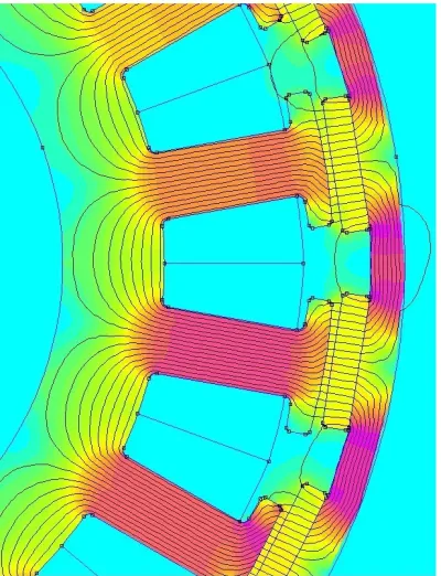
3.7 Flux density distribution in a motor. Darker colours correspond to
higher flux density. . . 44
3.9 Motor structure. The combined area of a slot and a tooth body is
enclosed in the yellow contour. The combined weight of the magnet and steel material enclosed by the red contour scales proportionally
to the weight of the tooth body. . . 54
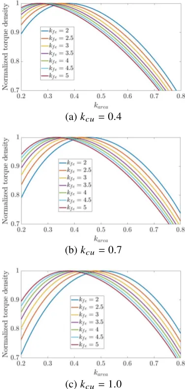
3.10 Plots of normalized motor torque againstkar eafor different values of kf eandkcu . . . 55 3.11 Colour bar of magnetic flux density for all FEA simulations in this
chapter. . . 58
3.12 Amplitude of the fundamental frequency (on left) and THD (on right)
of the motor phase bEMF for a range of values for the magnet width,
wm, and tooth tip width,wtip, both inmm. . . 59 3.13 Amplitude of the fundamental frequency (on left) and THD (on right)
of the flux density in the center of a motor stator tooth for a range of
values for the magnet width,wm, and tooth tip width,wtip, both inmm. 59 3.14 Motor phase bEMF (on left) and tooth flux density (on right) for a
range of values for the magnet width, wm, and tooth tip width, wtip,
both inmm. . . 60 3.15 Amplitude of the fundamental frequency (on left) and THD (on right)
of the motor phase bEMF for a range of values for the magnet width,
wm, and tooth tip width, wtip, both inmm. The body width of the teeth is chosen such that saturation occurs. . . 60
3.16 Motor phase bEMF (on left) and tooth flux density (on right) for a
range of values for the magnet width, wm, and representative tooth
tip width, both inmm. The body width is chosen such that saturation occurs. . . 61
3.17 Plot of phase bEMF harmonic content of the motor design
corre-sponding to the yellow curves in the plots of Fig. 3.15. . . 61
3.18 FEA simulations, showing the flux density levels in the motor for
different values for the magnet width, wm, and tooth tip width,wtip, both inmm. . . 62 3.19 Electro-Magnetic FEA simulation of the two motors of Table 3.1.
The motor withq =24 slots is shown on the left and the motor with q=30 slots is shown on the right. . . 64 3.20 Flux density at tooth center for the two motors with q = 24 and
3.21 Electro-Magnetic FEA simulation of the two motors of Table 3.2.
The motor withq =48 slots is shown on the left and the motor with q = 54 slots is shown on the right. Flux lines are not shown due to the small size of the teeth. . . 66
3.22 FEA simulation results comparing motors that have the same stator
outer diameter. The plots on the left show how the number of poles
affects the motor torque, torque density and efficiency for different
stator inner diameters. The figures on the right show the flux density
distribution in representative motor designs. . . 68
3.23 Motor losses as a function of motor speed for the design of Fig. 3.22f. 69
3.24 Motor normalized inductance as a function of the pole count for different values of the motor inner diameter. . . 69
3.25 Electro-magnetic FEA simulations of a SMPM motor and an IPM
motor that have the same outer diameter. The characteristics of the
motors are compared in Table 3.3. . . 71
3.26 First EV motor prototype. . . 73
3.27 Second EV motor prototype. . . 73
3.28 Early EV prototype FEA losses prediction as a function of motor speed at load of 5.5N m. . . 74 3.29 Motor cogging torque plots for a range of values for the stator outer
diameter, dout, and the tooth tip width, wtip, both in mm. The right plot focuses on a design region of lower cogging torque. . . 75
3.30 Motor average torque (on left) and motor torque ripple (on right) for
a range of values for the stator outer diameter,dout, and the tooth tip width,wtip, both inmm. . . 76 3.31 Motor torque density for a range of values for the stator outer diameter,
dout, and the tooth tip width,wtip, both inmm. . . 76 3.32 Final EV motor prototype that uses the 14 pole - 12 slot configuration
to improve the motor core losses. . . 77 3.33 Phase-to-phase bEMF voltage wave form for the motor of Fig. 3.32
at 3500RPM. FEA simulation prediction is compared to measured
experimental data. . . 78
3.34 Robotics motor prototype that has 60 poles and 54 slots. . . 78
3.35 Robotics motor prototype FEA losses prediction as a function of
3.36 Phase-to-phase bEMF voltage wave form for the motor of Fig. 3.34
at 1000RPM. FEA simulation prediction is compared to measured
experimental data. . . 79
3.37 Performance comparison of the motors (square symbol) developed in this section with off-the-shelf high performance frameless motors. 80 3.38 Motor scaling modes. The referent motor is a 20 pole-18 outer rotor motor. The pole scaled motor has 40 pole-36 slot motor configuration, which is quite popular in the drone industry (see Fig. 3.3.) . . . 81
4.1 Harmonic drive [88] ©2003 IEEE. . . 94
4.2 Cycloidal drive [95] ©2012 IEEE. . . 94
4.3 One-stage planetary gearbox [99] ©2011 IEEE . . . 95
4.4 Single stage compound planetary gearbox examples ([31] ©2018 IEEE on left and [32] ©2017 IEEE on right). . . 95
4.5 Wolfrom planetary gearbox layout [90] ©2009 Springer and CAD rendering. . . 97
4.6 Forces in Wolfrom Gearbox. . . 100
4.7 Compound planet side view. . . 102
4.8 Gear Bearing Drive [101] ©2018 Springer. . . 104
4.9 Example gearbox design with tooth correction. Left: CAD rendering. Right: 3D printed prototype. . . 105
4.10 Example gearbox design without a sun gear. Left: CAD rendering. Right: 3D printed joint prototype that features the gearbox. . . 106
4.11 The Bearingless Planetary Gearbox kinematic layout (one left) and CAD rendeing (on right). . . 107
4.12 Bearingless planetary gear drive prototype. Right: prototype show-ing the floatshow-ing nature of all components. Left: prototype in 3D printed case that axially constraints the motion of the gears. The gearbox diameter and width are 170mm and 23.175mm, while the driving sun gear diameter is 90mm. The weight is 1.1 Kg. . . 109
4.14 Left: plane gear forces due to meshing with ring gear and sun gear
in the bearingless planetary gearbox. F is the tangential meshing force (corresponding to Fg or Ff) and αis the gear pressure angle. Middle: two sided contact between a planet gear and a sun gear.
Right: clearance in the meshing between the ring gears and the sun
gears due to gearing backlash. . . 110
4.15 Planet meshing contact loads of the bearingless planetary gearbox. . . 111
4.16 Contact pressure distribution in the meshing between the planet gears
and the ring gears in the bearingless planetary gearbox, neglecting
the effect of the airgap. The peaks of the two distributions for the
planet gearszf andzgare 2Ff
b and 2Fg
b , respectively. . . 112 4.17 FEA model and mesh of Wolfrom gearbox (on left) and bearingless
planetar gearbox (on right). For both gearboxes, the sun and ring
gears are constrained to rotate around their centers. A load of 25N m is applied to both gearbox ring gears (supported by only one planet).
The planet of the bearingless planetary gearbox is floating while the
planet of the Wolfrom gearbox is constrained so that it may only
rotate around its axis. . . 114
4.18 FEA simulation results for the stress distribution in the planet gears
due to the meshing with the ring gears for the Wolfrom gearbox (on left) and bearingless planetary gearbox (on right). A load of 25N m is applied to both gearbox ring gears (supported by only one planet).
The stress in the ring gears is not shown because it is lower than the
stress in the planet gears, as predicted by the analysis of Sec. 4.2.3. . 114
4.19 FEA simulation results for the stress distribution in the planet gears
due to the meshing with the sun gears for the bearingless
plane-tary gearbox (on right). Exaggerated FEA simulation views of the
deformation are shown in the middle and on the right. . . 115
4.20 FEA simulation model and mesh (on left), and simulation results (on right) for the stress distribution in the planet gears due to the meshing
with the ring gears for the bearingless planetary gearbox with thinner
ring gears. . . 116
4.22 Prototype of the bearingless planetary gearbox with no planet
assem-bly features. The gearbox on the left is a remake of the gearbox of Fig. 4.12 with substantially lower backlash and is used in the actuator
prototype of Sec. 6.3. The gearbox on the right has reduction ration
of 1 : 10 and is used in the actuator prototype of Sec. 6.2. . . 120
4.23 Schematic construction of a backlash-free bearingless planetary gear-box with five assembled planets. . . 121
4.24 Prototype of a bearingless planetary gearbox with assembled planets. It is used in the actuator prototype of Sec. 6.4 . . . 122
4.25 Assembled bearingless planetary gearbox planet design. . . 123
5.1 Linear springs based designs. Left [10] ©2009 IEEE and right [9] ©2005 Springer. . . 126
5.2 Previous Spiral Spring Designs. . . 127
5.3 Planar rotary spring structure. . . 129
5.4 Curved beam kinematics [111] ©2011 Springer. . . 130
5.5 Spring arm kinematics. . . 131
5.6 Kinematics of the spring arm’s deformation. . . 132
5.7 Composite material spring arm. The sandwich structure on the left, its cross-section in the middle and its transformed section on the right. 135 5.8 Spring arm cutouts. . . 137
5.9 Deformations of the spring that cause the arms to intersect. . . 139
5.10 Spring design search Results. Left: torque at maximum displacement ∆β. Right: maximum bending stress at maximum displacement∆β. . 140
5.11 AR500 spring profile. . . 140
5.12 Spring torque loading components vs. displacement. . . 141
5.13 AR500 Spring design. . . 142
5.14 AR500 spring prototype. . . 143
5.15 FEA AR500 spring simulation results at maximum spring torsional loading. Counterclockwise loading on the left and clockwise loading on the right. The colour bar units correspond to stress in M Pa. . . . 144
5.16 AR500 spring experimental testing set-up. A close view of the spring on the right and the ADMET testing machine on the left. . . 145
5.17 AR500 spring mechanical torsion test experimental data. A plot of torque against angular displacement on the left and a combined plot of torque and angular displacement against time on the right. . . 145
5.19 Stress against displacement plot for the AR500 spring. . . 146
5.20 Titanium spring prototype on the left and its half section view on the right. . . 148
5.21 Contacting spiral arms. . . 150
5.22 Spring arm loading forces. . . 150
5.23 Spring arm interference and contacts initial guess. . . 152
5.24 FEA torsional simulation of the titanium spring prototype of Sec. 5.2.7155 5.25 Spring arm differential element along the neutral surface. . . 156
5.26 Spring composite arm structure. . . 158
5.27 Optimized spring shape. The curves trace the arm neutral surfaces. . 160
5.28 Spring shape with constant in-plane thickness. . . 165
5.29 Spring arm bending stress at displacement β. . . 165
5.30 Uni-directionally optimized spring shape. . . 166
5.31 Uni-directionally optimized in-plane spring arm thickness d. . . 166
5.32 Spring arm bending stress for uni-directionally optimized spring at displacements∆βmax and−∆βmax. . . 167
5.33 Bi-directionally optimized spring shape. . . 167
5.34 Bi-directionally optimized in-plane spring arm thicknessd. . . 167
5.35 Spring arm bending stress for bi-directionally optimized spring at displacements∆βmax and−∆βmax. . . 168
5.36 7075 Al spring prototype. . . 169
5.37 7075 Aluminum spring prototype torsional testing. . . 169
5.38 FEA simulation results at design spring torsional loading. Counter-clockwise loading on the left and Counter-clockwise loading on the right. The colour bar units correspond to stress in M Pa. . . 170
5.39 Spring torque against displacement plot. . . 170
5.40 Maximum arm bending stress against displacement plot. . . 171
6.1 Low reduction (1 : 10) bearingless planetary gearbox on left and modified driving outer rotor motor on right. The motor rotor is incorporated into the gearbox driving sun gear. . . 175
6.2 Low reduction actuator prototype. On left: complete assembly. On right: with output case removed. . . 175
6.3 Section views the low reduction actuator prototype. . . 176
[image:14.612.114.506.59.721.2]6.5 Bearingless series elastic actuator prototype. Fig. 6.6 shows the
actuator schematic structure. . . 178 6.6 Bearingless series elastic actuator structure. . . 179
6.7 Axel rover at field tests. The tether managements system is
high-lighted in the red circle (middle picture). . . 180
6.8 Axel primary tension module. Top: CAD section views of
mecha-nism [36] ©2018 IEEE. Bottom: Photographs showing the components.180
LIST OF TABLES
Number Page
3.1 Characteristics of two motors that have the same number of poles,
p= 28, and main dimensions but different number of slots. . . 63 3.2 Characteristics of two motors that have the same number of poles,
p = 56, and main dimensions but different number of slots. Flux lines are not shown due to the small stator tooth size. . . 65
3.3 Characteristics of a SMPM motor and IPM motors that have the
same outside diameter, and pole and slot count. The slot depth of
each motor is FEA optimised for maximum torque density (see Sec.
NOMENCLATURE
(Fxend,Fyend). Ch. 5: Spring arm end forces.
(Fx,Fy). Ch. 5: Spring arm loading. May have superscripts if spring deformation in both directions is concerned.
(xc,yc). Ch. 5: Coordinates of spring arm centroid surface in the plane.
(xn,yn). Ch. 5: Coordinates of spring arm neutral surface in the plane.
(xdis,ydis). Ch. 5: Displacement of spring arm distal end.
[σ]. Ch. 5: Spring material maximum admissible stress.
α. Ch. 5: Tangent angle of spring arm neutral surface.
β0. Ch. 5: Angular position of spring arm distal end.
δβ. Ch. 5: Incremental angle in spring displacement simulation.
∆d. Ch. 5: Spring primary material layer thickness.
∆E. Ch. 5: Spring stiffness reduction due to composite structure.
∆M. Ch. 5: Spring mass reduction due to composite structure.
∆β. Ch. 5: Spring displacement.
∆βmax. Ch. 5: Spring specified maximum displacement.
δcoor d,δdir. Ch. 5: Termination constants for spring arm contact locations update.
ηH,ηF. Ch. 4: bearingless planetary gearbox strength dertating constants.
γ. Ch. 5: Spring arm neutral surface displacement. May have subscript if spring deformation in both directions is concerned.
µ. Ch. 5: Spring material coefficient of friction.
µj
i. Ch. 1: joint friction coefficient of thei
t h joint in the jt h limb.
µ0. Ch. 3: Permeability of free space.
µR. Ch. 3: Relative permeability of rare earth magnets.
νa. Ch. 4: tangential velocity of driving sun gear in gearbox.
ωa. Ch. 4: angular velocity of driving sun gear in gearbox.
ωr ated. Ch. 3: Motor rated rotational speed.
Φc. Ch. 3: Amplitude of armature reaction flux.
Ψ. Ch. 3: Amplitude of motor phase flux linkage.
ψ(.). Ch. 3: Motor phase flux linkage.
ρ. Ch. 5: Spring material density.
ρs. Ch. 5: Spring secondary material density.
ρcu. Ch. 3: Density of copper.
ρf e. Ch. 3: Density of steel.
σ. Ch. 3: Motor winding resistivity.
σ. Ch. 5: Spring arm bending stress.
σF,σH. Ch. 4: bending/Hertz stress in gearbox.
σy. Ch. 5: Spring material yield strength.
σ[F],σ[H]. Ch. 4: maximum admissible bending/Hertz stress of gear material in gearbox.
σcv. Ch. 5: Spring arm bending stress on concave surface.
σcx. Ch. 5: Spring arm bending stress on convex surface.
σmax. Ch. 5: Spring arm maximum bending stress.
τ. Ch. 5: Spring torque.
τa, τl, τf,τg. Ch. 4: gear meshing torques in bearingless planetary gearbox.
τi. Ch. 1: it h joint torque in manipulator or limb.
τdes. Ch. 5: Spring specified maximum torque.
θ. Ch. 5: Polar location of spring arm centroid surface,θ ∈ [θmin, θmax].
θi. Ch. 1: it h joint angle in manipulator or limb.
Θij. Ch. 1: actuator output angle of theit h joint in the jt h limb.
θm. Ch. 3: Motor rotor mechanical angle of rotation.
ξi. Ch. 1: it h joint twist in manipulator or limb.
ζj
i . Ch. 1: actuator friction coefficient of thei
t h joint in the jt h limb.
a. Ch. 5: Radius of curvature of pring arm inner (convex) surface.
Ag. Ch. 1: floating base acceleration.
ag. Ch. 3: Motor air gap thickness.
Aslot. Ch. 3: Motor slot area.
Atot. Ch. 3: Combined area of a slot and tooth of motor stator.
b. Ch. 4: gear out-of-plane thickness in gearbox.
b. Ch. 5: Radius of curvature of spring arms outer (concave) surface.
Bc. Ch. 3: Amplitude of armature reaction flux density.
Bg. Ch. 3: Motor air gap flux density.
Bq. Ch. 3: Peak flux density in the motor stator tooth.
Br. Ch. 3: Motor magnet residual flux density.
c,q. Ch. 5: Spring archimedean spiral arm coefficients.
C0. Ch. 1: floating base frame. cf. Ch. 3: Motor slot fill factor.
CF,CH. Ch. 4: gear strength factors in gearbox.
Ci. Ch. 1: frame fixed to linkiin manipulator or limb.
cl. Ch. 3: Motor lamination fill factor.
Cq(q). Ch. 3: Motor slot factor.
CR,Ckc,CAq,CAs. Ch. 3: Motor slot analysis related geometric constants.
Cs. Ch. 3: Motor scaling factor.
Cw. Ch. 3: Motor winding factor.
d. Ch. 5: Spring arm in-plane thickness.
de. Ch. 4: gearbox ring gear diameter.
df. Ch. 4: gearbox planet gear diameter.
ds. Ch. 5: Spring secondary material layer thickness.
din. Ch. 3: Motor stator inner diameter.
dwir e. Ch. 3: Motor bare copper wire diameter.
dm. Ch. 5: Mass of spring arm differential element.
E. Ch. 5: Young’s modulus of spring material.
e. Ch. 5: Spring arm eccentricity.
Es. Ch. 5: Spring secondary material Young’s modulus.
fcoor d,fdir. Ch. 5: Discrete recursive filters for spring arm contact locations update.
fe. Ch. 3: Motor electrical frequency.
Ff,Fg,Fa. Ch. 4: gear meshing forces in gearbox.
Fi. Ch. 1: wrench between linkiand linki−1 in manipulator or limb.
g. Ch. 4: greatest common divider ofzezg−zbzf andzgin gearbox.
gi−1,i. Ch. 1: rigid body transformation of frame Ci relative to frame Ci − 1 in manipulator or limb.
h. Ch. 4: gearbox carrier.
Ii. Ch. 1: it h joint reflected inertia in manipulator or limb.
Im. Ch. 3: Motor synchronous current.
Jm. Ch. 3: Motor rotor inertia.
K. Ch. 5: Spring stiffness.
kA. Ch. 3: Motor axial scaling coefficient.
kc. Ch. 3: Motor winding coefficient.
Kd. Ch. 5: Spring arm scaled thickness.
Kh,Ke,Ka. Ch. 3: Motor core loss coefficients.
kP. Ch. 3: Motor pole scaling coefficient.
kq. Ch. 3: Motor topology family order.
kR. Ch. 3: Motor radial scaling coefficient.
ks. Ch. 3: Motor slot-pole symmetry.
ks. Ch. 5: Spring composite structure design trade-off.
Kt. Ch. 3: Motor torque constant.
kar ea. Ch. 3: Ratio of motor tooth body area to slot area.
kcu. Ch. 3: Windings mass coefficient.
Kdes. Ch. 5: Spring specified stiffness.
kf e. Ch. 3: Ratio of the combined mass of the rotor, the stator teeth and yoke to the mass of the body of the teeth of a motor.
Kph. Ch. 3: Motor phase bEMF constant.
L. Ch. 5: Spring arm length along the neutral surface.
lm. Ch. 3: Motor out-of-plane thickness.
lt. Ch. 3: Length of motor tooth.
Lkg. Ch. 3: Motor phase leakage inductance.
Lph. Ch. 3: Motor phase inductance.
Ls f. Ch. 3: Motor phase self inductance.
Ls. Ch. 3: Motor synchronous inductance.
M. Ch. 5: Moment in spring arm.
m. Ch. 4: module of gears.
Mi. Ch. 1: it h link generalized inertia matrix in manipulator or limb.
Mcen. Ch. 1: robot generalized inertia matrix in the given configuration.
Mdyn. Ch. 1: generalized inertia matrix of manipulator or robot (neglecting actuator reflected inertia).
Mm. Ch. 3: Motor mass.
Mr ob. Ch. 1: generalized inertia matrix of manipulator or robot.
N. Ch. 5: Spring arm shear force.
n. Ch. 1: number of links in manipulator or limb.
n. Ch. 5: Spring arm count.
Ncoor d. Ch. 5: Spring arm contact locations.
Ndir. Ch. 5: Spring arm contact force direction.
Nc. Ch. 5: Spring arm contact force.
Nturns. Ch. 3: Motor number of winding turns per stator tooth.
P. Ch. 3: Motor base topology pole count.
p. Ch. 3: Motor pole count.
Ph,Pe,Pa. Ch. 3: Motor core loss components.
pL. Ch. 3: motor pole count threshold value at which Ls f = Lkg.
pn. Ch. 4: number of planets in gearbox.
Pco. Ch. 3: Motor core loss.
Pcu. Ch. 3: Motor rated copper loss at stall.
Q. Ch. 3: Motor base topology slot count.
q. Ch. 3: Motor slot count.
Qpp. Ch. 3: Motor slot per pole per phase.
R. Ch. 5: Location of spring arm centroid surface in polar coordinates.
r. Ch. 5: Spring arm radius of curvaturer ∈ [a,b].
rc. Ch. 5: Radius of curvature of spring arm centroid surface.
Rn. Ch. 5: Radius of spring arm distal end.
rn. Ch. 5: Radius of curvature of spring arm neutral surface.
Rs. Ch. 3: Motor synchronous resistance.
rw. Ch. 3: Motor average winding radius.
Rae. Ch. 4: gearbox reduction ratio.
Rag. Ch. 3: Motor air gap reluctance.
Rin. Ch. 5: Radius of spring inner circle.
Rm. Ch. 3: Motor magnet reluctance.
Rout. Ch. 5: Radius of spring outer circle.
Rphase. Ch. 3: Motor phase resistance.
Rslot. Ch. 3: Motor slot resistance.
Rterm. Ch. 3: Motor terminal resistance.
s1,s2. Ch. 5: Spring arm contact positions along the neutral surface.
Sij. Ch. 1: the compliant element spring constant of theit h joint in the jt hlimb.
t. Ch. 5: Spring out-of-plane thickness.
Te. Ch. 4: gearbox output torque.
Tf. Ch. 4: gearbox planet torque at output ring gear.
Tm. Ch. 3: Motor torque.
tm. Ch. 3: Motor magnet thickness.
tr. Ch. 5: Spring transformed section thickness.
ts. Ch. 5: Spring arm secondary material layer thickness.
Tρ. Ch. 3: Motor torque density.
Tpeak. Ch. 3: Motor peak torque.
ttip. Ch. 3: Motor stator tooth tip thickness.
U. Ch. 5: Strain energy of spring arm differential element.
Um. Ch. 5: Strain energy density of spring arm differential element.
Vi. Ch. 1: it h link velocity in manipulator or limb.
Vr ated. Ch. 3: Motor rated voltage.
wt. Ch. 3: In-plane thickness of the motor stator teeth.
wtip. Ch. 3: Width of the tips of the teeth of a motor stator.
yr. Ch. 3: Motor rotor yoke.
ys. Ch. 3: Motor stator yoke thickness.
za. Ch. 4: driving sun gear or number of teeth of the driving sun gear in gearbox.
ze,zb,. Ch. 4: ring gear or number of teeth of ring gear in gearbox.
zf,zg,. Ch. 4: planet gear or number of teeth of planet gear in gearbox.
C h a p t e r 1
INTRODUCTION
1.1 Robotics Actuation
The majority of robotic systems are actuated using electric motors. Hydraulically
and pneumatically actuated robots also exist, however, these are rare due to their
control challenges, high cost and lower efficiency as a pump or compressor needs
to supply constant fluid pressure during operation. Furthermore, the usually high
pressures require regular maintenance and pose safety concerns during operation.
The design of a robot that features partial hydraulic actuation is described in [1]. A
pneumatically actuated bipedal is described in [2]. A classical comparative study
of robotics actuator technology is available in [3]. This thesis is concerned with the
design of robotic actuators featuring electric motors.
It is well known that electric motors with high power density that significantly
exceeds biological muscle may be readily designed. However, such power levels
are achieved only at very high rotational speed as motor torque density is quite low
[3, 4]. The electro-magnetic torque limitations of motors are fundamental, thus,
reaching the high torque levels needed for robotic joints requires the introduction of
a speed reducer between the motor and the load.
Outstanding torque amplification may be achieved with compact and light gearboxes such as harmonic drives and cycloidal drives (their advantageous and disadvantages
are outlined in Ch. 4). Even though actuators consisting of electric motors coupled
with high reduction gearboxes are very common, they suffer from very high reflected
inertia and no backdrivability, therefore, these actuators may not tolerate unexpected
shocks, and robot impacts with the environment may lead to permanent damage.
A popular approach to increase the shock tolerance of an actuator that features a high
reduction gearbox is to include a compliant element between the gearbox output and the load. The result is a series elastic actuator (SEA) [5]. Since the introduction of
the idea, many prismatic [6–8] and rotary [9–16] series elastic actuator designs have
been presented. Fig. 1.1 shows examples of prismatic and rotary SEA designs.
The rotation of the screw or gearbox output causes deformation of the elastic element
spring stiffness allows for an accurate estimation of the actuator force or torque to
be obtained so that joint level force control may be implemented. Furthermore, significant energy may be stored in the elastic element deformation, thus, improving
the robot operational efficiency during cyclic motion. These advantages of SEAs
come at the price of significantly reduced achievable force or torque control
band-width, typically not exceeding 10H z. SEA robot design, control, implementation
Figure 1.1: Examples of prismatic [8] ©2014 IEEE and rotary [17] ©2015 IEEE series elastic actuator designs.
and prototyping are described in [6, 7, 18–29].
SEA humanoid robots are predominantly controlled under static equilibrium. High
performance controlled dynamic manipulation and locomotion using SEAs has not
been shown to date.
SEA quadruped robots are either controlled under static equilibrium, similar to SEA
humanoids, or using dynamic trot gaits where the feet placement accuracy is low
and the actuators inject energy every cycle to maintain a bouncing-like locomotion.
It is the author’s opinion that the SEA robot performance limitations are intrinsic
and related to increased dynamics sensitivity caused by the actuators’ elasticity,
which may not be overcome using advanced control strategies. Ch. 2 shows
how the actuator reflected inertia impacts the dynamic sensitivity of robots, and in
particular, shows that series elasticity eliminates its potential dynamics benefits.
Recently, an alternative approach to robot actuation design has been developed.
Rather than using small motors running at high speed coupled with high reduction
gearboxes, large torque-optimized motors are coupled with low to mid reduction
ratio gearboxes. The resulting actuators may have good gearbox transparency and
backdrivability with much higher bandwidth than SEAs. However, due to the
need to dissipate significantly higher amount of heat to deliver the same amount
of static torque compared to SEAs of the same size. As shown in Ch. 2, low to mid reduction ratio geared actuators may also reduce a robot’s intrinsic dynamics
sensitivity to a minimum level. MIT’s Cheetah [4, 30] is an example of a quadruped
robot design which is actuated with low reduction gearboxes (one stage planetary)
coupled with high torque (off-the-shelf frameless) motors. Unmatched dynamic
capability with great robustness has been demonstrated with this robotic system. A
possibly improved actuator design that features mid reduction ratio gearbox (one
stage compound planetary) with high torque (off-the-shelf frameless) motors is
[image:26.612.305.504.266.423.2]introduced in [31, 32].
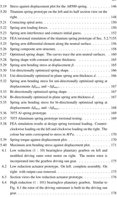
Figure 1.2: Robosimina: NASA Jet Prop.
Lab. entry to DRC [33] ©2015 Wiley. Of main interest in this thesis are limbed
or legged robots that have more than
two limbs so that some of the limbs are
used for manipulation or locomotion (or
both). The primary motivation is
Ro-boSimian (Fig. 1.2) which is DARPA
Robotics Challenge (DRC) entry of
NASA Jet Prop. Lab. RoboSimian has
28 degree-of-freedom (DOF) and four limbs that are capable of both mobility
and manipulation [33]. All robot
ac-tuators are identical and each feature a
harmonic drive with 1 : 160 reduction ratio with no added elasticity. Thus,
Ro-boSimian is mainly designed for stable, quasi-static locomotion and manipulation
with limited shock tolerance and impacts with the environment may result in
per-manent damage. Furthermore, the harmonic drive nonlinearities and friction (Sec.
4.1) prevent implementation of joint-level force control. An objective of this
the-sis is to investigate alternative approaches to the actuation of multi-limbed robots (such as RoboSimian) that feature improved shock tolerance and allow joint-level
force control so that dynamic locomotion and manipulation may be implemented on
1.2 Dual Robotic Actuation
The SEA shortcomings may be overcome by introducing a new robotic joint
archi-tecture that couples a low to mid reduction ratio geared motor to the SEA in parallel.
In the resulting dual actuator:
• the SEA would store energy, and produce static and low bandwidth torque
efficiently with low heat dissipation.
• the low to mid reduction ratio geared motor would produce high bandwidth
torque and reduce robot dynamics sensitivity. The high frequency torque
would generally be of lower amplitude, thus, the contribution of the low to
mid reduction ratio geared motor to the total loss is expected to be low, despite
its generally lower torque production efficiency.
The novel dual actuator can potentially preserve the shock tolerance of SEAs,
pro-vided the low to mid reduction ratio gearbox has high efficiency and backdrivability.
A dual actuation approach has been proposed in the past [34, 35]. In this previous work, the SEA is positioned away from the robotic joint at the base and is cable
coupled in parallel to a direct drive joint motor. The main disadvantage of this
approach is that the direct drive motor does not contribute with reflected inertia, and
thus, does not reduce the robot dynamics sensitivity (see Ch. 2). Also due to the
lack of a gearbox, the direct drive motor may only deliver limited torque with high
energy dissipation.
The main motivation and goal of the work presented in this thesis is to enable the
development of high performance actuation for legged, limbed and mobile robots. Due to the fact that such robots need to support their own weight, their actuators
need to be light weight, compact and efficient. Towards this goal high torque density
electric motors are developed in Ch. 3, a novel light weight and compact bearingless
planetary gearbox is introduced in Ch. 4 and torque density optimized SEA rotary
1.3 Thesis Structure and Contributions
Ch. 2 provides an analysis of robot dynamics sensitivity and shows how actuator
re-flected inertia impacts it in manipulators, and limbed and legged robots. The analytic
results motivate the proposed dual actuation approach. Open chain manipulators
(Sec. 2.2), and limbed/legged robots (Sec. 2.3) designed with geared actuators
are considered. Series elastic actuators are considered in Sec. 2.4. Example robot models are analyzed in Sec. 2.5.
Ch. 3 is concerned with the design and prototyping of high performance
per-manent magnet motors. Sec. 3.2 discusses the application-specific motor design
requirements for electric vehicles (Sec. 3.2.1), drones (Sec. 3.2.2) and robotic joint
actuators (Sec. 3.2.3). Sec. 3.3 describes the structure of permanent magnet motors
and outlines the advantages of outer rotor motors with concentrated windings. Sec.
3.3.3 describes a flux linkage model for these motors which is used in the derivation
of the analytic design trade-offs and guidelines of Sec. 3.4. Sec. 3.4.1 describes how a motor’s slot count affects its performance, Sec. 3.4.2 discusses high pole
count motors in the context of high speed applications, Sec. 3.4.3 introduced motor
design trade-offs characteristic of motors with high pole count and Sec. 3.4.4
dis-cusses how the tooth width and area may be optimized to improve a motor’s torque
and torque density. Next, Sec. 3.5 provides electro-magnetic FEA verification of
the results of Sec. 3.4 and Sec. 3.6 describes the development and fabrication of
motor prototypes, designed according to the proposed guidelines and methodology.
Finally, Sec. 3.7 describes the possible motor scaling modes and discusses the
challenges and limitations related to the practical implementation of high torque motors.
Ch. 4 is concerned with the design and prototyping of high torque, compact, and
lightweight gearboxes for robotic applications. Sec. 4.2 is concerned with the
anal-ysis, design and manufacturing of the Wolfrom Gearbox and introduces important
practical improvements. This gearbox is attractive due to its wide range of
reduc-tion ratios. Sec. 4.3 describes the development of a novel Bearingless Planetary
Gearbox which is the main contribution of the chapter. Detailed strength analysis
and manufacturing considerations are included in order to outline its advantages in terms of torque, weight, compactness and manufacturing readiness. The gearbox is
unique for its floating components and lack of carrier and bearings.
Ch. 5 is concerned with the analysis, design, and prototyping of rotary planar
proposes a systematic planar rotary spring modeling and analysis procedure. A
new mathematical model for multi-armed rotary springs with significant lattitude in the arm design is presented (Sec. 5.2.2). Two methods for spring mass reduction,
based on composite materials orcutouts, are introduced (Sec. 5.2.4). The design, manufacturing and testing of two spiral spring prototypes based on the proposed
analytical model are described (Sec. 5.2.6 and Sec. 5.2.7). Sec. 5.3 discusses
internal spring arm contacts. A systematic model of arm contacts is first introduced
(Sec. 5.3.1). Then, a complete spring torsional analysis algorithm that accounts for
arm contacts is presented (Sec. 5.3.2). Sec. 5.4 presents a consistent
optimization-based spring design procedure. The optimization-optimization-based approach is first motivated
(Sec. 5.4.1). Then, a complete optimization-based spring design algorithms is presented (Sec. 5.4.2). Finally, the design, analysis and testing of an aluminum
spring prototype are described (Sec. 5.4.3).
Ch. 6 describes actuator prototypes that feature components developed according
to the approaches of Ch. 3, Ch. 4 and Ch. 5. Sec. 6.2 describes an actuator that
features a 1 : 10 reduction ratio bearingless planetary gearbox. Sec. 6.3 describes
a series elastic actuator that features a 1 : 101 reduction ratio bearingless planetary
gearbox and an elastic element designed according to Ch. 5. Sec. 6.4 describes a
C h a p t e r 2
ROBOT DYNAMICS SENSITIVITY
2.1 Introduction
This chapter defines and analyzes the dynamics sensitivity of multi-limbed robots
and shows how their actuator designs impact this sensitivity. It is shown that the
reflected inertia of a multi-limbed robot’s actuators may improve the condition
number of the generalized mass matrix, thus, reducing its sensitivity to joint torque
errors. Both open chain manipulators (Sec. 2.2), and limbed/legged robots (Sec.
2.3) are considered and some important differences are outlined. These lead to
implications regarding robot design with geared actuators and series elastic actuators
(Sec. 2.4). Example robot models are analyzed in Sec. 2.5.
A crucial design aspect that is usually neglected in robot design is the robot’s
gen-eralized mass matrix dependence on the actuators’ characteristics. This chapter
provides a brief derivation of a robot’s inverse dynamics using Newton-Euler
re-cursive algorithm. The classical result for an open chain manipulator [37–39], is
extended to a floating base dynamics formulation for limbed and legged robots.
The close form dynamics equations allow a natural robot generalized mass matrix
decomposition that reveals the dependence of its condition number on the actuator
properties, e.g. actuator reflected inertia.
The condition number of a robot’s mass matrix is of great significance for torque
controlled robots because it determines how joint torque errors are propagated to
joint acceleration errors. A high condition number signifies that relatively small
joint torque errors in a subset of the robot’s joints may lead to unexpected large
acceleration errors in a possibly different subset of joints. This is demonstrated in
Sec. 2.5, where mass matrix analysis is provided for a 12 DOF quadruped robot
model and for RoboSimian (see Sec. 1.1). In the case of high mass matrix condition number, fast robot motion or heavy loading of its end effectors may lead to large
unstable oscillations that span most of the robot’s joints under closed loop control.
Therefore, a robot’s generalized mass matrix condition number provides a strong
indication of the robot’s dynamic capabilities.
The derivations begins with the assumption of geared motor type actuators, that is,
SEAs are considered in Sec. 2.4. Fig. 2.1 shows an example two-link robot
manipulator with joints driven by geared motors. The analysis of this section uses screw theory and the notation developed in [40].
Figure 2.1: A two-link robot arm driven by gearmotors [37] ©2008 Springer.
2.2 Open Chain Manipulator Inverse Dynamics
First, an open chain manipulator that consists of rigid body links connected by
one-degree of freedom revolute joints is considered. Fig. 2.2 shows the structure
Figure 2.2: Open chain manipulator structure.
The following definitions are used in the rest of the chapter:
• τi is theit h joint torque,
• gi−1,iis the rigid body transformation of frameCirelative to frameCi−1,
• ξi is theit h joint twist,
• θi is theit h joint angle,
• Miis theit hlink generalized inertia matrix,
• Viis theit h link velocity.
The base acceleration is defined asVÛ0 = Ag because in the case of a manipulator, the base acceleration is used to account for gravity.
The Newton-Euler recursive dynamics algorithm is given by [37, 38]:
• Forward Recursion:
Vi = Adg−1
i−1,iVi+ξiθiÛ
Û
Vi = ξiθiÜ + Adg−1
i−1,iVÛi−adξiθÛi(Adg−1i−1,iVi).
(2.1)
• Backward Recursion:
Fi= AdgT−1
i,i+1
Fi+1+MiVÛi−adVTiMiVi
τi= ξT
i Fi.
(2.2)
The adjoint transformation, Adgi,j transforms twists and wrenches from referencei
frame to reference frame j[40]. For a given twistξ =
h
ν ωiT,
adξ =
"
ˆ
ω νˆ
0 ωˆ
#
.
As shown in [39], the Newton-Euler recursive dynamics formulation may be written
in a matrix form:
MdynθÜ+K A0+LFn+1+C =τ, where
Mdyn =ξTGTMGξ
K = ξTGTMGP0 L= ξTGTPtT
C= ξTG(MG(P0Ag+adξθÛP0V0+adξθÛΓV)+adVTMV).
The various matrices in Eq. (2.3) have the following definitions: V = V1 ... Vn
∈ R6n, θÛ=
Û θ1 ... Û θn
∈ Rn, F =
F1 ... Fn
∈R6n, ξ =
ξ1 0 0
0 . . . 0
0 0 ξn
∈ R6n×n
P0 =
Adg−01,1 0 ... 0
∈ R6n×6, Pt =
0 . . . 0
Adg−1n,n+1
T
∈ R6×6n, τ=
τ1 ... τn
∈ Rn,
M=
M1 0 . . . 0
0 M2 . . . 0
... ... ... ...
0 0 . . . Mn
, G =
I 0 . . . 0 0
Adg−11,2 I . . . 0 0
... ... . . . ... ...
Adg−11,n Adg−21,n . . . Adg−n1−1,n I
, Γ =
0 0 . . . 0 0
Adg−11,2 0 . . . 0 0
... ... ... ... ...
0 0 . . . Adg−1n−1,n 0
, adξθÛ =
−adξ1θ1Û 0 . . . 0
0 −adξ2θÛ2 . . . 0
... ... . . . ...
0 0 . . . −adξnθÛn
,
adVT =
−adVT
1 0 . . . 0
0 −adVT
2 . . . 0
... ... . . . ...
0 0 . . . −adVT
n , (2.4)
whereM,G,Γ,adξθÛ andadVT ∈R6n×6n.
As discussed in [37], Eq. (2.3) can be very sensitive. This is demonstrated by showing that 0.5% error on the joint torques may lead to more than 40% error on the joint accelerations of an example 6 DOF planar arm that has identical joints
and links. This sensitivity may be explained by considering the manipulator’s
generalized mass matrix, Mdyn. Mdyn is a symmetric positive definite matrix [40] that can have a very high condition number in some configurations, especially
for manipulators with many DOF. For symmetric positive definite matrices, the
condition number is defined as κ(Mdyn) =
σ1(Mdyn)
σn(Mdyn) =
λmax(Mdyn)
λmin(Mdyn), where σj(Mdyn)
may propagate to large acceleration errors, and in this case, Eq. (2.3) becomes an
ill-conditioned problem for the accelerations. In this case, injecting relatively small magnitude torque in the joint space direction of the minimum eigenvalue of the mass
matrix may lead to very large accelerations in the same joint space direction.
In the derivation of Eq. (2.3), the actuator reflected inertia is neglected. In order
to introduce its dynamics effects, let Ii be the it h joint reflected inertia and I =
diag(I1, . . . ,In). The updated backward recursion from Eq. (2.2) is given by:
Fi = AdT g−1
i,i+1
(Fi+1−Ii+1ξi+1θiÜ+1)+MiVÛi+ξiIiθiÜ −adVTiMiVi
τi =ξT
i Fi.
(2.5)
Thus, the updated mass matrix in Eq. (2.3) becomes:
Mr ob= Mdyn+ξTIξ = Mdyn+I. (2.6)
All robot joints are assumed to be either revolute or prismatic, otherwiseξTIξ = I is not valid. Next, of main interest is howI affects the condition number, κ(Mr ob). Due to the fact that both Mdynand I are positive definite, the condition number of Mr obis bounded by:
κ(Mr ob)6
λmax(Mdyn)+max
i Ii
λmin(Mdyn)+min
i Ii
. (2.7)
Eq. (2.7) suggests that the reflected actuator inertia may be used to modify the
condition number of the mass matrix, and thus, the sensitivity of the dynamics
problem described in Eq. (2.3).
For example, if one designs the actuators so that they all have the same reflected
inertia, which is equal to the maximum eigenvalue of the mass matrix (I1 = · · · = In = λmax(Mdyn)), thenκ(Mr ob) 6 2. This condition may often be achieved using geared motors with low to mid reduction ratio.
For manipulators with ”stiff” actuators, that, is actuators that feature high reduction
gearboxes, it is usually the cases thatλmax(Mdyn) min
i Ii. Then,Mr ob ≈ Iand the actuators’ reflected inertia overshadows the manipulator dynamics. This effect may
be used to explain the high positional accuracy of ”stiff” manipulators. Due to their
high reflected inertia, disturbances and unmodeled dynamics have little effect on the
joint acceleration, that is, the dynamics coupling between the joints is effectively
high accuracy positioning control. However, the high actuator reflected inertia leads
to high impedance (Mr ob≈ IandImay be quite large), thus, the loading and forces that results from contacts of the manipulator with the environment may be very high
and unexpected impacts may lead to substantial damage.
2.3 Limbed and Legged Robot Inverse Dynamics
This section considers limbed and legged robots that are constructed by attachingk open chain manipulator limbs (legs and/or arms) to a central body (a floating base).
Most bipedal and quadruped robots may be modeled in this way. The equations of
motion for such robots may be derived by extending the backwards recursion in the
Newton-Euler algorithm to the floating base. For the jt h limb, the variables and matrices in Eq. (2.3) and Eq. (2.4) are given with superscript j. The floating base acceleration is defined asVÛ0 = A0 + Ag so that gravity is again compensated for, while A0is the actual acceleration ofC0. Let M0 be the generalized inertia matrix of the central body. Then, extending the backward recursion to the floating base
leads to the Newton-Euler equation for the central body:
M0A0− AdVT0M0V0+ k
Õ
j=1 Ad−T
g0j,1(F j 1 −ξ
j 1I
j 1θ
j
1)+ M0Ag= 0. (2.8)
Expanding and rewriting leads to the robot dynamics equations:
(M0+ k
Õ
j=1
M0j)A0+ k
Õ
j=1
KjθÜj + k
Õ
j=1
L0jFnj+1+C0+ k
Õ
j=1
C0j = 0 (2.9)
(K1)TA0+(M1+ I1) Üθ1+L1Fn1+1+C i = τ1
...
(Kk)TA0+(Mk+Ik) Üθk +LkFk n+1+C
k = τk.
(2.10)
Where,
Mj =(ξj)T(Gj)TMjGjξj, Kj = (P0j)T(Gj)TMjGjξj, Lj =(ξj)T(Gj)T(Ptj)T,
Cj =(ξj)TGj(AdVTjM
j
Vj+MjGj(P0jAg+AdξjθÛjP
j
0V0+ AdξjθÛjΓ
j Vj)
M0j =(P0j)T(Gj)TMjGjP0j, L0j =(P0j)T(Gj)T(Ptj)T,
C0j =(P0j)T(Gj)T(AdVTjM
j
Vj +MjGj(P0jAg+ AdξjθÛjP
j
0V0+AdξjθÛjΓ j
Vj))
C0=−AdVT0M0V0+M0Ag.
Eq. (2.9) describes the actuated dynamics and Eq. (2.10) describes the unactuated
dynamics of the robot. Then, the robot’s generalized mass matrix is:
Mr ob=
Mcen K1 . . . Kk
(K1)T M1 0. . . 0
... ... ... ...
(Kk)T 0 0. . . Mk
| {z }
Mdyn +
0 0 . . . 0
0 I1 0. . . 0
... ... ... ...
0 0 0. . . Ik
, (2.12)
where, Mcen = M0+Ík
j=1M j
0 is the inertia matrix of the robot (all the links and central body) in the given configuration w.r.tC0. Similar to open chain manipulators, the mass matrix Mdyn may have a very high condition number, κ(Mdyn). Let K =
h
K1 . . . Kk
i
, Mlim = diag(M1, . . . ,Mk), Ilim = diag(I1, . . . ,Ik). Mr ob,
Mdyn, Mlim andMcenare symmetric positive definite [40] and have complete set of orthogonal eigenvectors that span their respective joint space. Then, Mr ob can be factored using the Schur decomposition:
Mr ob=
"
Mcen K
KT Mlim
# + " 0 0 0 Ilim # = " 1 0
KTMcen−1 1
# "
Mcen 0
0 Mlim−KTMcen−1K
# "
1 Mcen−1K
0 1 # + " 0 0 0 Ilim # = " 1 0
KTMcen−1 1
#
| {z }
YT
"
Mcen 0
0 Mlim+Ilim−KTMcen−1K
#
| {z }
X
"
1 Mcen−1K
0 1
#
| {z }
Y .
(2.13)
Defining X andY matrices according to Eq. (2.13) leads toκ(Mr ob)6 κ(Y)2κ(X), therefore,
κ(Mr ob)6 κ(Y)2max(λmax(Mcen), λmax(Mlim+Ilim−K
TM−1 cenK))
min(λmin(Mcen), λmin(Mlim+Ilim−KTMcenK−1 )) . (2.14)
Alternatively:
"
1 0
−KTMcen−1 1
#
| {z }
Y−T
"
Mcen K
KT Mlim+Ilim
# "
1 −Mcen−1K
0 1
#
| {z }
Y−1
=
"
Mcen 0
0 Mlim+Ilim−KTMcen−1K
#
| {z }
X
.
Therefore:
κ(Mr ob)> κ(Y−1)−2max(λmax(Mcen), λmax(Mlim+Ilim−K
TM−1 cenK))
min(λmin(Mcen), λmin(Mlim+Ilim−KTM−1
cenK))
. (2.16)
Eq. (2.14) and Eq. (2.16) provide upper and lower bounds for the robot mass matrix
condition number as a function of the actuator reflected inertia matrix Ilim. The matrix K describes how the actuated dynamics in Eq. (2.9) affects the unactuated dynamics in Eq. (2.10) and vice versa. Thus, the matrices Mcen−1K1 . . . Mcen−1Kk describe how joint angle accelerations of each of the limbs propagate to acceleration
of the total robot mass and inertia. The matrices(K1)TMcen−1Kj. . . (K2)TMcen−1Kj. . .
(Kk)TMcen−1Kj describe how the resulting accelerations of the total robot mass and inertia, due to accelerations of the joints in the jt h limb, map to torques in the joints of all robot limbs. Therefore, for most robot designs that have at least two limbs and
significant fraction of their mass concentrated in their central base, one can expect
thatkKTMcen−1kandkKTMcen−1Kkare low (in most caseskKTMcen−1k,kKTMcen−1Kk <<
1). Then, Eq. (2.14) and Eq. (2.16) suggest that the robot’s generalized mass matrix
condition number may be approximated as:
κ(Mr ob) ≈ max(λmax(Mcen), λmax(Mlim+Ilim))
min(λmin(Mcen), λmin(Mlim+Ilim)) . (2.17)
Eq. (2.17) suggests that similar to open chain manipulators, a proper choice of the
actuators’ reflected inertia may improve a robot’s generalize mass matrix condition
number, κ(Mr ob), by improving the condition number of the actuated dynamics portion, which corresponds to the limbs. However, the portion of the mass matrix
that corresponds to the unactuated dynamics remains mostly unaffected by the
actuators. Thus, unlike manipulators, the condition number of the mass matrix of
limbed or legged robots always depends explicitly on the robot’s mechanical design
regardless of the actuators’ properties, and Eq. (2.17) suggests that the unactuated
dynamics portion of the mass matrix, Mcen, places lower bound, given by κ(Mcen), on the robot mass matrix condition number,κ(Mr ob). Furthermore, if the actuators’ reflected inertia is very high: max
i,j (I j
i)>> λmax(Mcen), λmax(Mlim), which is the case
with high reduction ratio "stiff" gearmotors, Eq. (2.17) suggests that the robot’s mass
matrix condition numberκ(Mr ob)may be quite high as in this case:
κ(Mr ob) ≈
max i,j
(Iij)
λmin(Mcen).
Thus, unlike open chain manipulators, high actuator reflected inertia, may have
This observation may be used to explain why humanoid or limbed robots built
with high reduction ratio harmonic drives are predominantly controlled under static equilibrium.
In summary, the simple analysis of this section suggests that as far as the dynamics
of limbed or legged robots is concerned, the actuator reflected inertia has profound
implication on the achievable robot performance in dynamic applications. Unlike
open chain manipulators, both low and high reflected actuator inertia results in
increased dynamics sensitivity that may propagate and significantly amplify joint
torque errors. Furthermore, Eq. (2.17) suggests that for a given robot, the actuator design may be tuned so that the robot’s generalized mass matrix condition number, κ(Mr ob), is minimized, and thus, the robot’s joint torque sensitivity is reduced to a minimum. Thus, as far as geared motors are concerned, one should expect optimum
dynamic performance to be achieved with actuators that feature reduction ratios in
2.4 Robots with Series Elastic Actuators
As discussed earlier, series elastic actuators are typically constructed by attaching a
compliant element between the load and the output of a high reduction gearbox that
is driven by a small sized motor. The following definitions for theit hjoint in the jt h limb are used in this section:
• µij is the joint friction coefficient,
• ζij is the actuator friction coefficient,
• Θij is the actuator output angle,
• Sij is the stiffness values of the compliant element.
The actuated robot dynamics of Eq. (2.1) and the unactuated robot dynamics of Eq.
(2.2) become:
(M0+ k
Õ
j=1
M0j)A0+ k
Õ
j=1
KjθÜj+ k
Õ
j=1
L0jFnj+1+C0+ k
Õ
j=1
C0j =0 (2.18)
(K1)TA0+M1θÜ1+L1Fn1+1+C i =
S1(Θ1−θ1) − µ1θÛ1 ...
(Kk)TA0+MkθÜk+ LkFnk+1+C k =
Sk(Θk−θk) −µkθÛk.
(2.19)
I1ΘÜ1+ζ1ΘÛ1= τ1+S1(θ1−Θ1)
... IkΘÜk+ζkΘÛk = τk+
Sk(θk −Θk).
(2.20)
Eq. (2.18) describes the actuated dynamics and Eq. (2.19) describes the unactuated
dynamics of the robot, which is coupled to the actuator dynamics of Eq. (2.20)
through the elastic elements. In this case, the robot’s generalized mass matrix is
actuators’ reflected inertia. As previously discussed Mdyn would normally have a large condition number, especially in the case of high DOF robots. Therefore, one should expect SEA robots to suffer from high sensitivity and significant dynamic
performance limitations due to joint oscillatory behavior under closed loop control,
which results from the SEA characteristic elasticity. Eq. (2.19) suggests that
improving a SEA robot’s dynamic performance may be achieved by:
• Increasing the SEA stiffness which may lead to reduced amplitude of
oscilla-tions. However, this also leads to degraded force control resolution.
• Increasing the joint friction which may lead to damping of oscillations.
How-ever, this also leads to increased losses and potential heating issues.
Dynamics sensitivity issues are reported in [15] regarding NASA-JSC Valkyrie which is a series elastic actuated humanoid robot with 44 DOF. In the article, the
sensitivity of the robot’s control system to the dynamics model is attributed to low
friction of SEA joints. However, as shown in this section, the joint torque sensitivity
of the SEA robots is an intrinsic dynamics problem that may not be solved by the
addition of joint friction or SEA stiffness increase. These measure only "mask" the
![Figure 1.2: Robosimina: NASA Jet Prop.Lab. entry to DRC [33] ©2015 Wiley.](https://thumb-us.123doks.com/thumbv2/123dok_us/8814893.919997/26.612.305.504.266.423/figure-robosimina-nasa-jet-prop-lab-entry-wiley.webp)