R E S E A R C H
Open Access
Finite algorithms for the numerical
solutions of a class of nonlinear
complementarity problems
Hongru Xu
1and Jinping Zeng
2**Correspondence:
[email protected] 2College of Computer Science,
Dongguan University of Technology, Dongguan, Guangdong 523808, PR China Full list of author information is available at the end of the article
Abstract
In this paper, we reformulate a nonlinear complementarity problem or a mixed complementarity problem as a system of piecewise almost linear equations. The problems arise, for example, from the obstacle problems with a nonlinear source term or some contact problems. Based on the reformulated systems of the piecewise almost linear equations, we propose a class of semi-iterative algorithms to find the exact solution of the problems. We prove that the semi-iterative algorithms enjoy a nice monotone convergence property in the sense that subsets of the indices consisting of the indices, for which the corresponding components of the iterates violate the constraints, become smaller and smaller. Then the algorithms converge monotonically to the exact solutions of the problems in a finite number of steps. Some numerical experiments are presented to show the effectiveness of the proposed algorithms.
MSC: 90C33; 65H10; 90C53
Keywords: nonsmooth equations; finite algorithms; complementarity problem; mixed complementarity problem
1 Introduction
LetF:Rn→Rnbe a given function. The nonlinear complementarity problem, denoted by
NCP(F,φ), is to find anx∈Rnsuch that
x≥φ, F(x)≥, (x–φ)TF(x) = . (.) In this paper, we focus on problem (.), in which the functionFhas the form ofF(x) = Ax+(x), that is, we have the problem of finding anx∈Rnsuch that
x≥φ, Ax+(x)≥, (x–φ)TAx+(x)= , (.) whereA= (aij)∈Rn×nis a given matrix,φ= (φi)∈Rnis a given vector, and:Rn→Rnis a given diagonal differentiable mapping, that is, theith componentiof(x) is a function of theith variablexionly:
i=i(xi), i= , , . . . ,n.
We denote the above problem byALCP(A,,φ) and call it an almost linear complemen-tarity problem (see,e.g., []). Obviously, ifis a linear function,ALCP(A,,φ) reduces to a linear complementarity problem.
ALCP(A,,φ) has many applications, especially in engineering. For instance, it can be derived from the discrete simulations of Bratu obstacle problem [], which models the nonlinear diffusion phenomena taking place in combustion and in semiconductors, and of some free boundary problems with nonlinear source terms, which models the diffusion problems involving Michaelis-Menten or second order irreversible reactions [, ].
In the literature, one classical approach used for solving (.) consists of the linearized projected relaxation methods [, ]. They are known to be convergent and easy to imple-ment. However, their convergence rates depend crucially on the choice of the relaxation parameter and deteriorate heavily with mesh refinement. In order to improve the effi-ciency, later multigrid methods were proposed (e.g.see [–]) and domain decomposition methods (e.g.see [–]), in which the subproblems are generally linear complementarity problems and then preconditioners, widely used in the linear systems, may not be applied directly. Another efficient way to solve problem (.) is given by active set strategies (e.g. see [–]). To solve the linear complementarity problem, the basic iteration of the active set strategies consists of two steps. First, based on a certain active set method, the (mesh) domain is decomposed into active and inactive parts. Then a reduced linear system asso-ciated with the inactive set can be solved by using a fast linear system solver such as the multigrid method or the preconditioned conjugate gradient method. For instance, in [, ], two approaches were introduced, respectively, for the elliptic and the parabolic case, where the Lagrange multiplier strategy is used in order to express the problem as a higher dimension standard equality problem. In particular, in [] such a strategy is combined with a semi-iterative procedure based on a suitable successive update of the coincidence set (that is, the area where the solution touches the obstacle), while in [] the solution of the parabolic variational inequality is obtained as the limit of the solutions of a family of appropriately regularized nonlinear parabolic equations. Alternately, inexact semismooth Newton methods have been developed to solve problem (.) based on its semismooth re-formulation [–]. These algorithms are attractive because they converge rapidly from any sufficiently good initial iterate and the subproblems are also systems of equations.
In this paper, we will propose some semi-iterative algorithms for the numerical treat-ment of an almost linear unilateral obstacle problem or mixed completreat-mentarity prob-lem. The algorithms are obtained as applications of piecewise almost linear systems to the problem which can be considered as an extension of piecewise linear systems to the affine lower obstacle problem [–]. The algorithms do not require the use of Lagrange multipliers and the involved subproblems in the algorithms are systems of almost linear equations, whose dimensions are less thann, the dimension of the original problem. We prove that the proposed algorithms enjoy a nice global monotonic convergence property in the sense that the subsets of the indices consisting of the indices, for which the corre-sponding components of the iterates violate the constraints, become smaller and smaller. Then the iterates converge to the exact solution in a finite number of steps. The numerical examples presented indicate the effectiveness of the proposed algorithms.
its monotone and finite convergence in Section . In Section , semi-iterative algorithms are proposed for solving upper obstacle problems and mixed complementarity problems, respectively, via their PALS reformulations, and the monotone and finite convergence of the algorithms are also obtained. In Section we present some numerical examples to in-vestigate the efficiency of the algorithms. Finally, in Section , we give a few conclusions.
2 Some preliminaries
For any given vectorx∈Rn, let the diagonal functionPφ(x) be defined as
Pφ(x) =diag
pφ(x),pφ(x), . . . ,pφn(xn)
(.)
with
pφi(xi) = ⎧ ⎨ ⎩
, ifxi≥φi, , ifxi<φi,
i= , , . . . ,n.
It is easy to see the following result is true [].
Lemma .
Pφ(x)(x–φ) =max{x,φ}–φ and
I–Pφ(x)
(x–φ) =min{x,φ}–φ.
According to Lemma ., we have the following conclusion.
Lemma . Let x be the solution of the following nonsmooth equations:
I–Pφ(x) +APφ(x)
(x–φ) +Pφ(x)(x–φ) +φ
+Aφ= . (.)
Let y=Pφ(x)(x–φ) +φ=max{x,φ}.Then y is the solution of the almost linear
complemen-tarity problem(.).
Proof It is easy to check by Lemma . that
I–Pφ(x) +APφ(x)
(x–φ) +Pφ(x)(x–φ) +φ
+Aφ
=min{x,φ}–φ+Amax{x,φ}–φ+max{x,φ}+Aφ
=min{x,φ}–φ+Ay+(y). (.)
By (.),xis the solution of problem (.) equivalent toy=max{x,φ}satisfying
Ay+(y) =φ–min{x,φ}= –min{x–φ, },
which implies
and
(y–φ)TAy+(y)= –max{x–φ, }Tmin{x–φ, }= .
That is,yis the solution of problem (.).
Remark . For the linear complementarity problem
x≥φ, Ax–b≥, (x–φ)T(Ax–b) = , (.) problem (.) reduces to the following piecewise linear system (PLS):
I–Pφ(x) +APφ(x)
(x–φ) =b–Aφ.
3 A semi-iterative algorithm for obstacle problem (1.2)
It is to be noted that the left-hand side of system (.) is not everywhere differentiable even for smooth. Nevertheless, a semi-iterative algorithm for solving system (.) can be constructed as follows:
Algorithm . LetP=O. Setk:= .
Step: Solve the system of findingxk+, such that
I–Pk+APkxk+–φ+Pkxk+–φ+φ+Aφ= (.) with
Pk=Pφ
xk, k= , , . . . , (.)
wherePφis defined by (.).
Step: If (Pk+–Pk)(xk+–φ) = , lety=Pk(xk+–φ) +φ=max{xk+,φ}and stop. Oth-erwise, go to Step .
Step: Setk:=k+ and go to Step .
Remark . In Algorithm ., one needs to solve a system of nonlinear equations (.)
at each iteration. Since the nonlinearity ofF(x) =Ax+(x) occurs only in the diagonal function, (.) is a system of almost linear equations (see,e.g., []). Especially, when F(x) =Ax–b, Algorithm . reduces to the semi-iterative Newton type algorithm for the solution of the linear complementarity problem (.). In this algorithm, only a system of linear equations needs to be solved at each iteration. We refer to [] for more details.
Remark . Let
Ik= i:pki = and Jk= i:pki = .
Equation (.) can be rewritten as ⎧
⎨ ⎩
AIkIkxk+
Ik +Ik(xk+
Ik ) = –AIkJkφJk, xkJk+=φJk–AJkIkxk+
where AIJ denotes submatrix ofAconsisting ofaijwithi∈I,j∈J, andxI denotes the subvector ofxconsisting ofxiwithi∈I. Consequently, the main work in solving (.) is to solve a system of almost linear equations with dimensionnk=dim(Ik)≤n.
In order to prove the convergence of Algorithm ., some preliminary results are needed first (see,e.g., [, ]).
Lemma . Let A be an M-matrix.Then,for any diagonal matrix P,whose diagonals are
zeros or ones,the two matrices I–P+AP and I–P+PA are M-matrices,and therefore, (I– P+AP)–≥and(I–P+PA)–≥.Furthermore,for any nonnegative diagonal matrix,
the matrices I–P+AP+and I–P+PA+are M-matrices,and then(I–P+AP+)–≥
and(I–P+PA+)–≥. Define
P= P∈Rn×n:Pis a diagonal matrix with zeros or ones diagonals
and
¯
SP= x∈Rn:TP(x)≥
,
where
TP(x) = (I–P+AP)(x–φ) +
P(x–φ) +φ+Aφ.
LetAbe anM-matrix andi(i= , , . . . ,n) be monotonically nondecreasing functions. Then, for anyP∈P,TPis anM-function. In fact, for anyx∈Rnandy∈Rn, ifTP(x)≥ TP(y), we have
TP(x) –TP(y) = (I–P+AP)(x–y) +
P(x–φ) +φ–P(y–φ) +φ
=I–P+AP+P(x,y)
(x–y)
≥, (.)
where
P(x,y) =
∇Px+t(y–x)+ (I–P)φdtP (.)
is a diagonal matrix with nonnegative diagonals. By Lemma ., (I–P+AP+P(x,y))–≥, and hence by (.), we havex≥y, which implies the inverse isotone ofTP. On the other hand, for every pair of indicesi=j, and for everyx∈Rn, noting thatAP:=I–P+AP= (aPij) is anM-matrix,aPij≤. Therefore, the one-dimensional functiongijin the variablethas the form
gij(t) =
TP
xt,ji= l=j
aPil(xl–φl) +aPij(t–φj) +i
pi(xi–φi) +φi
+ n
j=
wherext,j= (x
, . . . ,xj–,t,xj+, . . . ,xn) andP=diag(p,p, . . . ,pn). It is clear thatgijis non-increasing, which implies the off-diagonal antitone ofTP. Therefore, the inverse isotone together with the off-diagonal antitone ofTPimplies thatTPis anM-function [].
For anyP∈Pandx∈ ¯SP, we have
≤TP(x) = (I–P+AP)(x–φ) +
P(x–φ) +φ+Aφ
=I–P+AP+P(x,φ)
(x–φ) +(φ) +Aφ,
whereP(x,φ) is defined as (.). Then,
I–P+AP+P(x,φ)
(x–φ)≥–(φ) –Aφ≥min –(φ) –Aφ, . Noting that (I–P+AP)–≥(I–P+AP+
P(x,φ))–≥ andmin{–(φ) –Aφ, } ≤ we have
x≥φ+I–P+AP+P(x,φ) –
min –(φ) –Aφ, ≥φ+ (I–P+AP)–min –(φ) –Aφ, .
That is,S¯Pis bounded below. On the other hand, letx=φ+ (I–P+AP)–max{–(φ) – Aφ, }. It is easy to checkx∈ ¯SP. In fact,
TP(x) =max –(φ) –Aφ,
+P(I–P+AP)–max –(φ) –Aφ, +φ+Aφ
≥max –(φ) –Aφ, +(φ) +Aφ≥,
by the use of the monotonicity ofand the relationP(I–P+AP)–max{–(φ) –Aφ, }+
φ≥φ. Therefore,S¯Pis nonempty and bounded below and has a minimal element. In fact, ¯
SP has unique minimal elementx∗P, which solvesTP(x) = ,i.e. TP(x∗P) = (see,e.g., [] and the references therein). According to the above discussion, we have immediately the following result.
Lemma . Let A be an M-matrix,andi(i= , , . . . ,n)be monotonically nondecreased functions.Then Algorithm.is well defined.
The following two lemmas are crucial for the convergence of Algorithm ..
Lemma . Let{Pk}be defined by(.).Then
Pk+–Pkxk+–φ≥, k= , , , . . . . (.)
Moreover,let{xk}be generated by Algorithm..Then,if the equality in(.)holds,xk+is
the solution of problem(.).
Proof Inequality (.) follows directly from the definitions (.) and (.). If for somek,
then, by (.),
I–Pk++APk+xk+–φ+Pk+xk+–φ+φ+Aφ
=I–Pk+APkxk+–φ+Pkxk+–φ+φ+Aφ, = ,
which implies thatxk+is the solution of problem (.).
Lemma . Let A be an M-matrix andi(i= , , . . . ,n)be monotonically nondecreased functions.Let{xk}and{Pk}be generated by Algorithm..Then
Pkxk+–φ≥Pk–xk–φ≥ · · · ≥Px–φ=O (.) and
Pk+≥Pk≥O, k= , , , . . . . (.)
Proof By (.), we have
=I–Pk+APkxk+–φ+Pkxk+–φ+φ+Aφ
=I–Pk–+APk–xk–φ+Pk–xk–φ+φ+Aφ. Therefore,
I–Pk+PkAPkxk+–φ+Pkxk+–φ+φ
=PkI–Pk+APkxk+–φ+Pkxk+–φ+φ
+I–PkPkxk+–φ+φ
=PkI–Pk–+APk–xk–φ+Pk–xk–φ+φ
+I–PkPkxk+–φ+φ
=I–Pk+PkAPk–xk–φ+Pk–xk–φ+φ
+Pk–Pk–xk–φ
+I–PkPkxk+–φ+φ–Pk–xk–φ+φ. (.) We note that ifpki = , thenxki <φiandpki = . It follows forpki = that
pkixki+–φi
+φi=φi and pki–
xki –φi
+φi≤φi. By the use of the monotonicity ofi, we have immediately
i
pkixki+–φi
+φi
–i
pki–xki –φi
+φi
≥, ifpki = ,
which implies
Equation (.) together with (.) and (.) leads to
I–Pk+PkAPkxk+–φ–Pk–xk–φ
+Pkxk+–φ+φ–Pk–xk–φ+φ
=I–Pk+PkA+kPkxk+–φ–Pk–xk–φ
≥, (.)
where
k=
∇Pk–xk–φ+φ+tPkxk+–φ–Pk–xk–φdt
is a diagonal matrix with nonnegative diagonals. By Lemma ., (I–Pk+PkA+k)–≥, and hence by (.), we getPk(xk+–φ) –Pk–(xk–φ)≥, that is, (.) holds.
Ifpk
i = ,xk≥φi, and by (.), we have xki+–φi=pki
xki+–φi
≥pki–xki –φi
≥.
This impliesxki+≥φiand hencepki+= =pik. Ifpki = , we immediately havepki+≥ =pki.
Therefore, we conclude (.).
Theorem . Let A be an M-matrix andi(i= , , . . . ,n)be monotonically nondecreased functions.Then Algorithm.is well defined and stops at the solution of problem(.)in a finite number of iterations.
Proof Lemma . implies that the algorithms are well defined. By Lemma . and Algo-rithm ., we haveI≥Pk+≥Pk≥ · · · ≥P=O. Obviously, we havePk+=Pk for some k<n. In this case, (Pk+–Pk)(xk+–φ) = . By Lemma ., we obtain the solution of the problem by Algorithm . within at mostnsteps.
Theorem . indicates that Algorithms . can obtain the solution of problem (.) within at mostnsteps. Nevertheless, the corresponding upper bound (i.e. n) may be large, when the dimension of the system is large. However, several numerical tests presented in Section show that the convergence can be reached in just a few iterations.
Define
S= x:min x–φ,Ax+(x)≤.
Then, if T(x) :=Ax+(x) is an M-function, the unique solution of problem (.) is the maximal element ofS(see,e.g., []). The following conclusion indicates that Algo-rithm . has a monotone convergence property.
Theorem . Let A be an M-matrix andi(i= , , . . . ,n)be monotonically nondecreased functions.Let{xk}and{Pk}be generated by Algorithm..Assume
Then{yk+} ⊂Sand
yk+≥yk≥ · · · ≥y.
That is to say,{yk}is inSand converges to the solution of problem(.)monotonically.
Proof The monotone convergence is from (.) directly. Ifyk+
i >φi,pki = , and by (.), we have
Ayk++yk+i
=I–Pk+APkxk+–φ+Pkxk+–φ+φ+Aφ+Pk–Ixk+–φ
i= ,
which impliesmin{yk+–φ,Ayk++(yk+)} ≤ andyk+∈S. In Theorem ., we assume thatAis anM-matrix. This assumption can be replaced by the following conditions:
nullAT≡span(v), null(A)≡span(w) and A+is anM-matrix (.) for somev> andw> (componentwise), and for any diagonal matrixsatisfying≥ and=O. This case may occur for elliptic problems with Neumann boundary condi-tion. Let furthervT(φ)≥. Similar to Lemma ., for any nonnegative diagonal ma-trix, and any diagonal matrixP=I, whose diagonals are zeros or ones, the matrices I–P+AP+andI–P+PA+areM-matrices, which imply (I–P+AP+)–≥ and (I–P+PA+)–≥ (see,e.g., []). According to the proof in Lemma ., forPk=I, problem (.) is well defined and (.) and (.) hold. IfPk=I=Pk–, we havexk≥φand thenPk–(xk–φ) +φ≥φ. By (.), we have
I–Pk–+APk–xk–φ+Pk–xk–φ+φ+Aφ= . Noting that
Pk–Pk–xk–φ=I–Pk–xk–φ≥, for positive vectorvgiven in (.), we have
≤vTPk–Pk–xk–φ
=vTI–Pk–xk–φ
=vTI–Pk–+APk–xk–φ
=vT–Aφ–Pk–xk–φ+φ
≤–vT(φ) ≤,
which implies (Pk–Pk–)(xk–φ) = , where the second inequality is fromv> ,null(AT)≡
Theorem . Let A satisfy(.)andi (i= , , . . . ,n)be monotonically nondecreased functions with vT(φ)≥.Then Algorithm.is well defined.Let{xk}and{Pk}be gener-ated by Algorithm.,and let
yk+=Pkxk+–φ+φ, k= , , , . . . .
Then{yk}is inSand converges monotonically to the solution of problem(.)in at most n iterations.
The above theorem also implies the existence of the solution for problem (.) under the conditions of Theorem ..
4 Some extensions
In this section, we make some extensions. First, let us consider the upper obstacle problem of finding anx∈Rnsuch that
x≤φ, Ax+(x)≤, (x–φ)TAx+(x)= , (.) whereA= (aij) is a given matrix,φ= (φi)∈Rnis a given vector, and:Rn→Rnis a given diagonal mapping defined as before.
For any given vectorx∈Rn, let the diagonal functionP
φ(x) be defined as
Pφ(x) =diag
pφ(x),pφ(x), . . . ,pφn(xn)
(.)
with
pφi(xi) = ⎧ ⎨ ⎩
, ifxi≤φi, , ifxi>φi.
Similar to Lemma ., we have the following lemma.
Lemma . Let x be the solution of the following nonsmooth equations:
I–Pφ(x) +APφ(x)
(x–φ) +Pφ(x)(x–φ) +φ
+Aφ= ,
where Pφ(x)is defined by(.).Then y=Pφ(x)(x–φ) +φ=min{x,φ}is the solution of the
almost linear upper obstacle problem(.).
According to Lemma ., a semi-iterative algorithm for solving upper obstacle problem (.) can be constructed as follows.
Algorithm . LetP=O. Setk:= .
Step: Solve the system findingxk+, such that
I–Pk+APkxk+–φ+Pkxk+–φ+φ+Aφ= , wherePk=P
Step: If (Pk+–Pk)(xk+–φ) = , lety=Pk(xk+–φ) +φ=min{xk+,φ}and stop. Other-wise, go to Step .
Step: Setk:=k+ and go to Step .
Similar to the proofs of Lemmas .-. as well as Theorems . and ., we have the following finite convergence result.
Theorem . Let A be an M-matrix andi(i= , , . . . ,n)be monotonically nondecreased functions.Then Algorithm.is well defined.Moreover,let{xk}and{Pk}be generated by Algorithm..Then
Pkxk+–φ≤Pk–xk–φ≤ · · · ≤Px–φ=O,
Pk+≥Pk≥O, k= , , , . . . ,
and
yk+≤yk≤ · · · ≤y,
where
yk+=Pkxk+–φ+φ, k= , , , . . . .
Therefore,Algorithm.stops at the solution of problem(.)in at most n iterations.
In the following, we consider the numerical solution of the almost linear mixed comple-mentarity problem of finding anx∈Rnsuch that (see,e.g., [])
⎧ ⎨ ⎩
xi≥φi, (Ax+(x))i≥, (xi–φi)T(Ax+(x))i= , ifi∈N,
(Ax+(x))i= , ifi∈N,
(.)
whereN∩N=∅andN∪N={, , . . . ,n}. Letϕ∈Rnbe any vector satisfying
ϕi=φi, ∀i∈N. (.)
For any given vectorx∈Rn, let the diagonal functionPϕ(x) be defined as
Pϕ(x) =diag
pϕ(x),pϕ(x), . . . ,pϕn(xn)
(.)
with
pϕi(xi) = ⎧ ⎪ ⎪ ⎨ ⎪ ⎪ ⎩
Noting that
APϕ(x)(x–ϕ) +Aϕ
i
=
j∈N,xj≥φj
aij(xj–ϕj) +
j∈N
aij(xj–ϕj) +
j∈N∪N
aijϕj
=
j∈N,xj≥φj aijxj+
j∈N,xj<φj aijφj+
j∈N
aijxj
and
Pϕ(x)(x–ϕ) +ϕ
i=
⎧ ⎪ ⎪ ⎨ ⎪ ⎪ ⎩
xi, j∈Nandxj≥φj,
φi, j∈Nandxj<φj, xi, j∈N,
the following result becomes obvious.
Lemma . Let x be the solution of the following nonsmooth equations:
I–Pϕ(x) +APϕ(x)
(x–ϕ) +Pϕ(x)(x–ϕ) +ϕ
+Aϕ= , (.)
where Pϕ(x)is defined by(.)andϕsatisfies(.).Then y=Pϕ(x)(x–ϕ) +ϕis the solution
of the almost linear mixed complementarity problem(.).
According to Lemma ., we construct the following algorithm for the solution of mixed complementarity problem (.).
Algorithm . LetP= (p i) with
pi = ⎧ ⎨ ⎩
, ifi∈N,
, ifi∈N.
Setk:= .
Step: Solve the system findingxk+, such that
I–Pk+APkxk+–ϕ+Pkxk+–ϕ+ϕ+Aϕ= , (.)
wherePk=P
ϕ(xk) is defined by (.) andϕsatisfies (.).
Step: If (Pk+–Pk)(xk+–ϕ) = , lety=Pk(xk+–ϕ) +ϕand stop. Otherwise, go to Step .
Step: Setk:=k+ and go to Step .
Similarly, we have the following conclusion.
Algorithm..Then
Pkxk+–ϕ–Pk–xk–ϕ≥O, i= , , . . . , Pk+≥Pk≥O, k= , , , . . . ,
and
yk+≥yk≥ · · · ≥y,
where
yk+=Pkxk+–φ+φ, k= , , , . . . .
Therefore,Algorithm.stops at the solution of problem(.)in at most n iterations.
For a matrixAsatisfying (.), the monotone and finite steps convergence can be de-duced in a similar way. We omit the details.
5 Numerical experiments
In this section, we present some numerical experiments in order to investigate the effi-ciency of the proposed algorithms. The programs are coded in Visual C++ . and run on a computer with . GHz CPU. We consider the following four problems.
Problem (Michaelis-Menten reaction []) We consider the following free boundary
problem on the unit square= (, )×(, ):
u–cut=f(x,y,u) +ε(x,y), u∈D,
wheref(x,y,u) =u/( +u),ε(x,y) is a local threshold consumption rate, andDis a domain in. At the free boundary (x=s(y)), the concentration and its gradient vanish. We take into account only the steady-state case,i.e.,c= with the following additional data on:
⎧ ⎪ ⎪ ⎨ ⎪ ⎪ ⎩
ε(x,y) = (y– .),
∂u
∂n= wheny= andy= ands(y) = , u(,y) =y( –y),
with x=s(y) being the free boundary. We shall be interested in a nonnegative solution of the above problem. We discretize the problem by using a five-point difference scheme with a constant mesh step size:h= /(m+ ), wheremdenotes the number of mesh nodes inx- ory-direction. Then Problem can be transformed to problem (.).
Problem ([]) We consider the following nonlinear complementarity problem:
Here,F(x) =Ax+D(x) +f, where
A= h ⎛ ⎜ ⎜ ⎜ ⎜ ⎜ ⎝
H –I
–I H . .. . .. ... –I
–I H ⎞ ⎟ ⎟ ⎟ ⎟ ⎟ ⎠ with H= ⎛ ⎜ ⎜ ⎜ ⎜ ⎜ ⎝ – – . .. . .. ... – – ⎞ ⎟ ⎟ ⎟ ⎟ ⎟ ⎠
andh=√
n+,D(x) = (Di) :R
n→Rnis a given diagonal mapping withD
i:R→R, fori= , , . . . ,n, that is, the componentDiofDis a function of theith variablexionly. SetDi(xi) =
λexi and obtain a diagonal mappingD(x) = (D
i(xi)). In our test, we fixλ= ., and let fi=max{,vi– .} ×wi–., wherewiandviare random numbers in [, ],i= , , . . . ,n.
Problem ([]) We discuss the following nonlinear complementarity problem:
x≥, F(x)≥, xTF(x) = ,
where
F(x) =Mx+D(x) +f.
The matrixM=ATA+Bis produced as follows. LetAbe ann×nmatrix whose en-tries are randomly generalized in the interval (–, ) and the skew-symmetric matrixBbe generated in the same way. Let the vectorf be generated from a uniform distribution in the interval (–, ). LetD(x) = (Di(xi)) :Rn→Rnbe a given diagonal mapping with Di(xi) =di∗arctan(xi),i= , , . . . ,n, wheredi(i= , , . . . ,n) are chosen randomly in (, ).
Problem (Signorini problem []) We consider the contact problem of finding ausuch
that ⎧ ⎪ ⎪ ⎨ ⎪ ⎪ ⎩
–u=f in= (, )×(, ),
u= onp={(x,y) :x= , ≤y≤} ∪ {(x,y) : ≤x≤,y= }, u≥, ∂∂un≥, ∂∂nuu= ons∪s,
wheres={(x,y) : ≤x≤,y= },s={(x,y) :x= , ≤y≤}, and
f(x,y) = ⎧ ⎨ ⎩
–, if (x,y)∈(, /]×(, ),
We discretize the problem by using a finite difference scheme with a constant mesh step size:h= /m, wheremdenotes the number of mesh nodes inx- ory-direction. Then Problem can be transformed to a linear mixed complementarity problem.
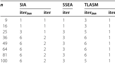
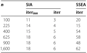
We compare different algorithms from the point of view of the iteration numbers. Here, we consider three algorithms: the semi-iterative algorithms proposed in this paper (de-noted by SIA), the semismooth equation approach proposed in [] (de(de-noted by SSEA), and two-level additive Schwarz method proposed in [] (denoted by TLASM).
For SIA, we choose the initial matrixP=Ofor all problems and adopt Newton iteration with line search to solve the system of nonlinear equations at each iteration. The termina-tion criterion of inner iteratermina-tion isαkdk
≤–, wheredkis the Newton direction and
αkis the step length. The number of inner iterations is denoted by iterinnand the iteration number of the algorithm is denoted by iter.
For SSEA proposed in [], we choose the initial pointx= , the parameters= –,
p= ,ρ= .,β= ..Hk∈∂Bis defined by the procedure proposed in Section of []. For TLASM, we use PSOR to solve all subproblems relating to obstacle problems with the tolerance –in·
norm. The systems of nonlinear equations in TLASM are solved by Newton iteration, and the termination criterion is the same as that in SIA. The relax-ation parameter in the relaxrelax-ation iterative method is chosen asω= .. In order to get a super-solution initial, we letx=A–e, withe= (, , . . . , )Tandx= –A–f, respectively, for Problems and . In TLASM, iterinnand iter are the same as that in SIA.
[image:15.595.196.396.473.585.2]It is easy to see from Tables - that the algorithms presented in this paper are com-petitive as regards the above three algorithms in most cases. As for TLASM, we need to find a super-solution initial of the problem, which may usually bring about some nu-merical difficulties. While compared with TLASM, it is much easier for SIA to choose a suitable initial point. Another advantage of SIA is that the subproblems in the algorithm
Table 1 Comparisons of iteration numbers for Problem 1
n SIA SSEA TLASM
iterinn iter iter iterinn iter
9 12 3 7 12 1
16 20 5 9 11 1
25 16 4 9 151 23
36 31 8 12 203 30
49 23 6 11 172 25
64 35 9 12 169 25
81 27 7 11 179 27
100 43 11 15 156 23
Table 2 Comparisons of iteration numbers for Problem 2
n SIA SSEA TLASM
iterinn iter iter iterinn iter
9 1 1 1 3 1
16 1 1 1 3 1
25 3 1 3 5 1
36 6 2 3 6 1
49 6 2 3 6 1
64 6 2 3 6 1
81 6 2 3 6 1
[image:15.595.197.396.620.730.2]Table 3 Comparisons of iteration numbers for Problem 3
n SIA SSEA
iterinn iter iter
100 11 3 20
225 14 4 15
400 15 5 54
625 18 6 58
900 18 6 48
1,600 18 6 62
Table 4 Algorithm 4.1 for Problem 4
n iter n iter n iter n iter
100 2 400 3 900 3 1,600 3
are systems of almost linear equations of dimensions less thann, while the subproblems in two-level additive Schwarz method still include complementarity problems. In Table , we do not list the results for two-level additive Schwarz method. The reason is that it is difficult for Problem to find a super-solution initial pointxand the algorithm may not converge. Theoretically, we may not guarantee the convergence of SIA for Problem since Ais not anM-matrix. However, it is interested to see from Table that SIA is still stable and effective since the iteration numbers are small and show almost no change with the increase of the dimension.
As for SSEA and TLASM, some modifications are needed in order to solve the mixed complementarity problems. So, we only run Algorithm . for Problem and the iteration numbers are listed in Table to solve the mixed complementarity problems with difference dimensions discretized by Problem . It is easy to see that Algorithm . is still effective for the problem.
6 Final remark
In this paper, we present some finite algorithms to the numerical solution of almost linear (mixed) complementarity problems. The algorithms are based on the systems of piecewise almost linear equations, which are the reformulations of the problems. It is proved that the algorithms converge monotonically to the solution of the problem in a finite number of steps. Indeed, we can produce a monotone lower solution or upper solution by iterates converging to the solutions of the problems by the algorithms. Numerical results show that the proposed method is effective.
Competing interests
The authors declare that they have no competing interests.
Authors’ contributions
All authors jointly worked on the results and they read and approved the final manuscript.
Author details
1School of Mathematics, Jiaying University, Meizhou, Guangdong 514015, PR China.2College of Computer Science,
Dongguan University of Technology, Dongguan, Guangdong 523808, PR China.
Acknowledgements
Received: 10 June 2015 Accepted: 6 August 2015
References
1. Wang, ZY, Fukushima, M: A finite algorithm for almost linear complementarity problems. Numer. Funct. Anal. Optim.
28, 1387-1403 (2007)
2. Rodrigues, JF: Obstacle Problems in Mathematical Physics. Elsevier, Amsterdam (1987)
3. Elliott, CM, Ockendon, JR: Weak and Variational Methods for Moving Boundary Problems. Research Notes in Mathematics, vol. 59. Pitman, London (1982)
4. Meyer, GH: Free boundary problems with nonlinear source terms. Numer. Math.43, 463-482 (1984)
5. Facchinei, F, Pang, JS: Finite-Dimensional Variational Inequalities and Complementarity Problems. Springer, New York (2003)
6. Glowinski, R: Lectures on Numerical Methods for Nonlinear Variational Problems. Springer, New York (1984) 7. Hackbusch, W, Mittelmann, H: On multigrid methods for variational inequalities. Numer. Math.42, 65-76 (1984) 8. Kornhuber, R: Monotone multigrid methods for elliptic variational inequalities I. Numer. Math.69, 167-184 (1994) 9. Zhang, Y: Multilevel projection algorithm for solving obstacle problems. Comput. Math. Appl.41, 1505-1513 (2001) 10. Badea, L, Tai, X, Wang, J: Convergence rate analysis of a multiplicative Schwarz method for variational inequalities.
SIAM J. Numer. Anal.41, 1052-1073 (2003)
11. Hoffmann, KH, Zou, J: Parallel solution of variational inequality problems with nonlinear source terms. IMA J. Numer. Anal.16, 31-45 (1996)
12. Jiang, YJ, Zeng, JP: A multiplicative Schwarz algorithm for the nonlinear complementarity problem with an
M-function. Bull. Aust. Math. Soc.82, 353-366 (2010)
13. Tai, XC: Rate of convergence for some constraint decomposition methods for nonlinear variational inequalities. Numer. Math.93, 755-786 (2003)
14. Tarvainen, P: Two-level Schwarz method for unilateral variational inequalities. IMA J. Numer. Anal.19, 273-290 (1999) 15. Zeng, JP, Zhou, SZ: Schwarz algorithm for the solution of variational inequalities with nonlinear source terms. Appl.
Math. Comput.97, 23-35 (1998)
16. Zeng, JP, Zhou, SZ: Domain decomposition methods and their convergence for solving variational inequalities with a nonlinear source term. Acta Math. Appl. Sin.23, 250-260 (2000)
17. Ito, K, Kunisch, K: Parabolic variational inequalities: the Lagrange multiplier approach. J. Math. Pures Appl.85, 415-449 (2006)
18. Kärkkänen, T, Kulisch, K, Tarvainen, P: Augmented Lagrangian active set methods for obstacle problems. J. Optim. Theory Appl.119, 499-533 (2003)
19. Xue, L, Cheng, XL: An algorithm for solving the obstacle problems. Comput. Math. Appl.48, 1651-1657 (2004) 20. Kanzow, C: Inexact semismooth Newton methods for large-scale complementarity problems. Optim. Methods Softw.
19, 309-325 (2004)
21. Sun, Z, Zeng, JP: A monotone semismooth Newton type method for a class of complementarity problems. J. Comput. Appl. Math.235, 1261-1274 (2011)
22. Sun, Z, Zeng, JP: A damped semismooth Newton method for mixed linear complementarity problems. Optim. Methods Softw.26, 187-205 (2011)
23. Sun, Z, Wu, L, Liu, Z: A damped semismooth Newton method for the Brugnano-Casulli piecewise linear system. BIT Numer. Math.55, 569-589 (2015)
24. Brugnano, L, Sestini, A: Numerical solution of obstacle and parabolic obstacle problems based on piecewise linear systems. AIP Conf. Proc.1168, 746-749 (2009)
25. Brugnano, L, Casulli, V: Iterative solution of piecewise linear systems and applications to flows in porous media. SIAM J. Sci. Comput.31, 1858-1873 (2009)
26. Brugnano, L, Casulli, V: Iterative solution of piecewise linear systems. SIAM J. Sci. Comput.30, 463-472 (2008) 27. Ortega, JM, Rheinboldt, WC: Iterative Solution of Nonlinear Equations in Several Variables. Academic Press, San Diego
(1970). Reprinted by SIAM, Philadelphia (2000)
28. Kikuchi, N, Oden, JT: Contact Problems in Elasticity: A Study of Variational Inequalities and Finite Element Methods. SIAM, Philadelphia (1988)
29. Noor, MA, Bnouhachem, A: Modified proximal-point method for nonlinear complementarity problems. J. Comput. Appl. Math.197, 395-405 (2006)
30. Walloth, M: Adaptive numerical simulation of contact problems: resolving local effects at the contact boundary in space and time. Diss. Universitäts und Landesbibliothek Bonn (2012)
31. Luca, TD, Facchinei, F, Kanzow, C: A semismooth equation approach to the solution of nonlinear complementarity problems. Math. Program.75, 407-439 (1996)
32. Xu, HR, Zeng, JP, Sun, Z: Two-level additive Schwarz algorithms for nonlinear complementarity problem with an