A Measure of the Proportion of Treatment Effect Explained by a Surrogate Marker

(1)

BIOMETRICS 58, 803-812 December 2002

A Measure of the Proportion of Treatment

Effect Explained by a

Surrogate Marker

Yue Wang* and Jeremy M.

G.

Taylor

Department

of Biostatistics, University

of Michigan,

1420 Washington Heights, Ann Arbor, Michigan 48109-2029, U S A .

*

email:

[email protected]

SUMMARY. Randomized clinical trials with rare primary endpoints or long duration times are costly. Be- cause of this, there has been increasing interest in replacing the true endpoint with an earlier measured marker. However, surrogate markers must be appropriately validated. A quantitative measure for the proportion of treatment effect explained by the marker in a specific trial is a useful concept. Freedman, Graubard, and Schatzkin (1992, Statistics in Medicine 11, 167-178) suggested such a measure of surrogacy by the ratio of regression coefficients for the treatment indicator from two separate models with or without adjusting for the surrogate marker. However, it has been shown that this measure is very variable and there is no guarantee that the two models both fit. In this article, we propose alternative measures of the proportion explained that adapts an idea in Tsiatis, DeGruttola, and Wulfsohn (1995, Journal of the American Sta- tistical Association 90, 27-37). The new measures require fewer assumptions in estimation and allow more flexibility in modeling. The estimates of these different measures are compared using data from an ophthalmology clinical trial and a series of simulation studies. The results suggest that the new measures are less variable.

KEY WORDS: Surrogate marker; Validation.

1. Introduction

Clinical trials with rare primary endpoints or long duration times often require large sample sizes and extensive periods of follow-up. Because of this, there has been increasing interest in using surrogate endpoints in lieu of the primary endpoints in these situations. Surrogate endpoints are usually intermediate biomarkers in disease development that can be observed and assessed earlier and are often easy t o measure. They are generally proposed based on the biological process of a disease and their strong correlations with the primary endpoint (El- lenberg and Hamilton, 1989; Schatzkin et al., 1990; Fleming, 1992). However, correlation alone is not a good statistical criterion for surrogate validation. For example, in AIDS-related trials, it is known that the levels of CD4 counts and virus load are associated with AIDS and death. But data suggest that treatment-induced improvements in CD4 or viral RNA load do not reliably predict treatment-induced changes in the primary clinical outcomes (Lagakos and Hoth, 1992; Fleming and DeMets, 1996).

Prentice (1989) proposed a formal definition of surrogate endpoints and gave general operational criteria for validation of the surrogate endpoints. By his criteria, an appropriate surrogate endpoint is required to fully capture the treatment effect on the primary endpoint. This is rather too stringent a criterion and is unlikely to be satisfied completely. In practice, it is likely that a surrogate endpoint may explain part but not all the treatment effect. However, the more explained, the

better we will perceive the marker as a surrogate endpoint. Thus, a quantitative measure of the proportion of the treatment effect that is explained by the surrogate marker would be a useful summary measure. For convenience, we refer to the proportion of the treatment effect explained by the biomarker as PE. Freedman, Graubard, and Schatzkin (1992) proposed such a quantitative measure for a single trial.

Daniels and Hughes (1997) proposed a meta-analysis nieth- od for the evaluation of a potential surrogate marker. A Bayes- ian approach was used to model the association between the treatment effects on the primary endpoints and the treatment effects on the surrogate endpoints from multiple clinical trials.

A marker is considered as a valid surrogate if the association is significantly different from zero. Their approach enables one t o obtain prediction intervals for the treatment effect on the primary outcome given the estimated treatment effect on the surrogate markers from a new trial.

Buyse et al. (2000) developed a new set of criteria for surrogate validation within the multiple clinical t.rial settings. They proposed a trial-level and an individual-level criteria. The trial-level criterion is the coefficient of determination

(2)

804

Biometrics, December

2002

ing notation is adopted: T and S denote the random variables for the primary endpoint and surrogate markers, respectively. 2 is the binary treatment indicator variable, with

Z

= 1 for treatment (or new treatment) and Z = 0 for placebo (or standard treatment). We will be assuming throughout the article that there is a treatment effect on the primary endpoint, i.e., P(T

1

2 )

#

P ( T ) , where P(.) denotes the probability distribution.

In a randomized clinical trial, a perfect surrogate occurs when S captures all the dependence of T on 2. In other words, P(T

I

2,s)

= P ( T

1

S ) . A useless surrogate can occur in cases where, conditional on the treatment assign- ments, the surrogate is independent of the primary endpoint, P ( T

I

2,s)

= P(T

I

2).

A useless surrogate can also occur when S is independent of the treatment indicator

Z,

P(S

I

2 ) = P(S). A partial surrogate occurs when the surrogate endpoint captures some but not all the dependence of T on

2.

An ideal measure of P E will be one for a perfect surrogate, zero for a useless surrogate, and between zero and one for a partial surrogate.

In Section 2, we review the quantitative measure for P E proposed by Freedman et al. (1992). In Section 3, we propose new measures for PE and investigate some of their properties. In Section 4, we discuss approaches to estimation and inference for the new measures. In Section 5 , data from a clinical trial in ophthalmology are used t o estimate the new measures and Freedman’s measure. In Section 6, simulation studies are carried out t o compare the new measures with Freedman’s measure in cases where T and S are binary.

2. Freedman’s Measure for Proportion of Treatment

Freedman et al. (1992) proposed a measure for PE within the context of a binary primary endpoint. The measure, denoted P , is defined based on two logistic models,

Effect Explained

and

and P =

( p

-

p ~ ) / , / 3

= 1

-

ps/p,

the difference between the treatment effect with or without adjusting for the surrogate marker divided by the unadjusted treatment effect. Assuming treatment has a significant effect on the primary outcome, then P = 1 if /!Is = 0 and P = 0 if

/!Is

=

p.

The measure P generalizes in obvious ways for other nonbinary variables T with appropriate models, e.g., time-to-event outcome with proportional hazard (PH) models.

Freedman’s P suffers a number of drawbacks (Daniels and Hughes, 1997; Lin, Fleming, and DeGruttola, 1997; Buyse and Molenberghs, 1998; Bycott and Taylor, 1998). First, models for [T

1

S , Z ] and [T

1

Z ] will be fitted simultaneously for estimation of P . However, in general, they will not both be true at the same time. Assuming the model for [T

I

S , Z ] is the correct one, integration with respect to P ( S

I

Z)

will not usually result in the exact linear form as the model for [T

I

Z]

except for a few special cases. Thus, in general, at least one model fitted will be misspecified. Lin et al. (1997) studied the behavior of estimated coefficients from misspecified PH models for censored failure time data.

Another drawback is that calculation of P requires there t o be no significant interaction term between the surrogate

S

and the treatment

2

in model (1). When the data suggest an interaction, P is not well defined. A third drawback for P to be a useful measure is that it has a large variability. TO get a reasonably precise estimate for P requires a highly significant unadjusted treatme$ effect or a large sample size. Otherwise, the point estimate P can lie outside [0,1] and the confidence interval for P frequently covers the whole [0,1] interval and is too wide t o be useful (Freedman et al., 1992; DeGruttola et al., 1996; Lin et al., 1997; Bycott and Taylor, 1998).

3. A New Measure for Proportion Explained

3.1 Definition of F

Tsiatis, DeGruttola, and Wulfsohn (1995) studied the relai tionship between survival and longitudinal CD4 counts. A model for the CD4 trajectory in each treatment group is developed. Let S ( t , Tr) and

S ( t ,

P1) denote the predicted survival curve in the treatment group and the placebo group, respectively. To see how much survival benefit could have been predicted by just the increase in CD4 counts, using the hazard function for the placebo group, the predicted survival curve S(t,mix) for an average CD4 trajectory from the treatment group was computed. If CD4 counts serve as a useful surrogate endpoint, S(t,rniz) would t o be close to S ( t , T r ) , whereas if changes in CD4 explain very little of the treatment effect, S(t,mix) would be close to S(t,Pl). The relative position of S ( t , mix) between S ( t , Tr) and S ( t , P1) was suggested as a way to assess the proportion of treatment effect explained.

Motivated by their work, we propose a new measure F for PE. We refer t o the placebo group

(Z

= 0) as group A and to the treatment group

(Z

= 1) as group B. The new measure is F = ( A A - A B ) / ( A A - B B ) , where A A = h(JgA(s)dPA(s)), B B = h(lgB(s)dPB(s)), and A B = h(/gA(S)dPB(S)). Here PA(S) and P B ( S ) denote the distribution of S in groups A and B, respectively. gA(S) and gB(S) are functions of the conditional distribution of T given S in the placebo and treatment groups, respectively. For example, gA

(S)

and gB ( S ) can be the mean of this distribution. h(.) is a monotonic function. In general, h ( . ) , gA(S), and g B ( S ) are chosen such that ( A A - B B ) will be the desired measure of treatment effect on the primary endpoint T.

To explain the idea, let T be a binary variable. Choose

h(u)

= u, gA(S) = P r ( T = 1

I

s,z

=

a),

and gB(S) =

P r ( T = 1

1

S , Z = 1). Then population quantities AA = P r ( T = 1

1

Z = 0) and B B = Pr(T = 1

1

Z = 1). The treatment effect ( A A - B B ) is the difference on the probability scale between the two groups. A A is the weighted mean of the conditional probability gA(S) with weight given by the density of S in the placebo group. Similarly, AB = i g A ( s ) d P ~ ( s ) is the weighted mean of gA(S) with the density of S in the treatment group as weight. Hence, AB measures what P r ( T = 1) in the placebo group would be if the values of the surrogate are distributed as those in the treatment group. If T = 1 represents disease occurrence, then A A - AB can be interpreted as the change in the risk that is due to the change in distribution of S induced by the treatment. A com- plementary form of F is F’ = ( B A - B B ) / ( A A - B B ) with

(3)

Use of Surrogate Markers

805

The choices of h ( . ) , gA(S), and gB(S) define the treatment effect. For binary T, we could express the treatment effect on the probability scale using h(u) = u as shown above. Alternatively, we could let h(u) = logu/(l -

u)

and g ( S ) =

P(T = 1

1

S ,

2)

if we believe the logit is the more natural scale on which t o assess probabilities. In this case, the treatment effect is expressed by log(odds ratio) with AA = logit[Pr(T =

1

[

Z

= O)] and B B = logit[Pr(T = 1

1

Z = l)]. For a time-to- event variable T, we may choose h(u) = u , gA(S) = P r ( T

>

c

I

S , z = 0) and gB(S) = Pr(T

>

c

1

S,Z = l), where c is a prespecified time, say 5 years. Then the treatment effect ( A A - B B ) is the difference in the probability of surviving at least 5 years between two groups. [image:3.616.318.559.80.245.2]

3.2 Conditions for Measure

to

Be Bounded Within [0,1] As a measure of proportion, we would prefer F and F’ to have values in the range from 0 t o 1 with 0 indicating a useless surrogate and 1 a perfect one. However, this i s not guaranteed. It is possible for F and F’ t o be less than 0 or greater than 1. In this section, we present and discuss the conditions for the population quantities F and F’ t o be bounded within [0,1]. We will also discuss situations where these population quantities will be outside [0,1]. By population quantities, we mean F and F‘ as functions of the joint distribution of T and S , which can be interpreted as the values that would arise from an infinitely large sample.

For simplicity, assume h(u) = u. For a perfect surrogate, the conditional distribution [T

I

S , Z ] is the same as

[T

I

S ] . Thus, gA(S) = g B ( S ) and F = F‘ = 1. For a useless surrogate, either

p ~ ( s )

=

p ~ ( s ) ,

or g A ( S ) and g B ( s ) are constant with respect to

S .

Both result in F = F’ = 0. Hence, for the perfect or useless scenario, the population quantities F and F’ are equal and take the desired values.

For a partial surrogate, in special cases, eg., when the treatment effect on T is not a function of

S ,

in other words, g A (S) = gB(S)+c where c is a constant, F will be equal t o F’. In general, F’ is likely t o have different values from F . As a measure of proportion, ideally, F and F’ will fall between zero and one in partial surrogate scenarios. However, this does not hold in all situations. Certain conditions need t o be satisfied for F and F‘ t o be bounded within (0,l).

Without the loss of generality, we assume A A

>

B B . Under this assumption, the conditions for F and

F’

t o be bounded within ( 0 , l ) are

These conditions are best understood in terms of a plot of gA(S) and gB(S) versus

S ,

as shown in Figure 1. [S

1

A] and [S

I

B ] are the distributions of the surrogate marker in groups

A and

B, respectively. g(S

1

2 ) is a function of the distribution of [T

I

S,

Z] for each value of 2. It could be the probability of disease or survivorship up to a certain time point or hazard at a certain time point. The position AA indicates approxim-

surrcgale markel

Figure 1. Illustration plot OfgA(S), gB(S) versus S. gA(S)

and gB(S) are functions of the conditional distributions of [T

[

S,Zl for group

A

(the placebo group) and group €3 (the treatment group). The solid line in the plot is gA(S) and the dashed line is gB(S). AA indicates the position that is approximately the value of E A [gA(S)]; similarly, AB approximates E B [ ~ A ( S ) ] , B A approximates E A [ ~ B ( S ) ] , and BB approximates E B [ g B ( S ) ] .

ately the value of E A [ ~ A ( S ) ] ; similarly, A B approximates E B [ g A ( S ) ] , B A approximates E A [gB ( S ) ] , and BB approximates E B [ ~ B ( S ) ] . For the perfect surrogate scenario, g A ( S ) = gB(s), and it is easy t o see F = F’ = 1 from the plot. For the useless surrogate scenario, either [S

1

Z

= 11 is identical t o

[s

I

z

= 01 or gA(S) and g B ( S ) become horizontal lines (constant with respect t o S ) . Both give F = F’ = 0. For the partial surrogate scenario, graphically what is required for both F and

F’

t o lie between zero and one is that both AB and B A lie between A A and B B .

The four necessary and sufficient conditions C1-C4 can be further simplified depending on the shape of gA(S) and gB(S) and the distributions of S in the two groups. Plots similar t o Figure 1 enable us to visualize relatively easily the necessary and sufficient conditions. Consider the cases where the distributions PA(S) and PB ( S ) have a stochastic ordering. Without loss of generality, assume PA(S) is stochastically higher than

P B ( S ) ,

i.e., Pr(S 5 s

1

group B)

2

Pr(S 5 s

1

group A) V s. It is easy t o see that

R1: PA(S)

stochastically higher than P B ( S )

R2: gA(S) and g B ( S ) are nondecreasing functions of

s

R3:

gA(S) - gB(S)

2

0 for all S

(4)

806

Biometries, December 2002

R1-R3 are simpler than Cl-C4 and are easier t o understand and check. Condition R1 is an assumption on how treatment affects the surrogate marker, and it is reasonable to think that it is satisfied for plausible markers being seriously considered in a randomized trial. Condition R2 is likely to be satisfied for any marker that is strongly associated with the primary endpoint. Condition R3 is the one that may not be satisfied in every trial. For example, if g A ( S ) and g B ( S ) represent the risk in the control and treatment groups, respectively, R3 requires that, conditioning on each value for the surrogate marker, the risk for the treated group should be consistently lower than the risk in the control group. R3 may not be true when there are unexpected aspects of the pathway between treatment, surrogate marker, arid primary endpoint. For example, unintended adverse effects can occur such that the risk is higher in the treated group than in the control group. In these cases, g A ( S ) is lower than g B ( S ) instead of higher, as shown in Figure 1. If the magnitude of the adverse effect is strong, A A - B B can be negative while AA - AB and B A - BB are positive due to R1 and R2. As a result, F and F’ have negative values. If the magnitude of the adverse effect is weak, A A - B B will be positive but less than A A - AB or B A

-

B B and results in values greater than one for F and In cases where conditions C1-C4 or Rl-R3 are satisfied, the scale from zero t o one corresponds t o a meaningful transition from useless surrogacy to perfect surrogacy. However, as described above, the population quantities F ( F’ ) can have values greater than one or less than zero, which most likely indicates the existence of unintended effects.

3.3 Interpretation of F (F’) in Special Cases

F is constructed based on the concept of trying to measure what the treatment effect would be if the surrogate marker in the nontreated group has the treatment-induced distribution and vice versa for F’. However, AB and B A are two hypothetical quantities that are not observable. In this section, we investigate F (8‘’) in several special situations where they can be represented by familiar quantities.

3.3.1 Normally distributed T and S . In cases where both T and S are normally distributed with linear mean structure, F‘.

si

= a0

+

a]ZZ

+

tS2

Ti

= yo

+

rizi

+

E T ~ ,

where

the model for T given ( S , Z ) is a linear model without an interaction term,

T =

Po

+

P1

s

+

P2Z

+

€*, where

OT

“S

Po

= y o - -Pff0, P1 = --P,

Pz

= 71 - - p a l , “T

US

*T

“ S

aST “SOT

’

P = ___

and

E* N N (0, a$ (1 - p ’ ) )

If we choose the treatment effect t o be the difference in mean, then

and

Thus, F (F’) depends on the strength of the association between T and S (measured by

P I ) ,

the effect of

Z

on S ( a l ) ,

and the adjusted treatment effect ( P 2 ) . In this example, the linear form of the mean structure for [T

I

Z ] can be obtained exactly by integrating E[T

I

S,Z]

with respect t o P ( S

1

2).

We note that

p = =

PlW

71

Pz

+ P l % ’

which is equal t o F ( F ’ ) . Also note that, in this case, condition R l is satisfied if

<

0 and R2 is satisfied if

01 2

0 and condition R3 is satisfied if P2 _< 0.

3.3.2 Binary primary endpoint and binary surrogate marker. Many diagnostic markers, with appropriate cutoff values, are used in medical applications t o predict disease. A good test would have high positive predictive value (PPV) and high negative predictive value (NPV). Let p + denote Pr(disease) and p - = 1 - pf

.

If a binary surrogate marker S is defined such that

S = { 1 if positive diagiiosis

and the treatment effect is the difference on the probability scale, then

F

= 6 y ~ / r and

F‘

= 6 7 B / 7 , where

0 otherwise

6 = P r ( S = 1

1

Z

= 0) - P r ( S = 1

I

2 = I ) , which is the treatment effect on S ,

7 = P r ( T = 1

1

Z

= 0) - Pr(T = 1

I

Z

= I ) ,

which is the treatment effect on T ,

y~ = P r ( T = 11 =

o,s=

1) - Pr(T= 1 [

Z

= 0,s =

o),

and

y~ = P r ( T = 1

I

Z

= 1,s = 1) - P r ( T = 1 j 2 =

1,s

= 0). Y A and y~ are equal t o [ ( P P V - p f )

+

( N P V - p - ) ] in the placebo group and the treatment group, respectively; thus, y

reflects the strength of the association between S and T , with larger y indicating higher association. F and F‘ are influenced by two components: the ratio of the treatment effect on S and T and the accuracy of the prediction of T based 011 S. For a

given treatment effect on the primary outcome ( T ) , the larger

(5)

Use of

Surrogate M a r k e r s

807

association between S and T, the higher F and F’ will be. The two components of F ( F ’ ) are very similar to the measures Buyse and Molenberghs (1998) proposed for surrogate validation, relative effect (RE) and adjusted association.

Condition R1 is satisfied if 6

>

0 and R2 is satisfied if YA

1

0 and Y B

2

0. R3 is satisfied if NPVA

5

NPVB and PPVA

2

PPVB, where ( N P V A , PPVA) and ( N P V B , PPVB) are the NPV and PPV in the placebo and treatment groups, respectively. Note in this case F = F’ if ( P P V

+

N P V ) are the same in the treatment and placebo groups.

3.3.3 Binary primary endpoint T. Now consider cases

where T is binary and the effect of S on T in group B is related to that for group A by a linear shift on the logistic scale. In other words,

logit(Pr(T = 1

1

S, Z ) ) =

Po

+PIS

- wZ.

Assume w to be a nonnegative constant so that treatment will reduce the odds of T = 1 given S = s. If we define the treatment effect (AA - BB) on the probability scale, then

which leads to messy expressions for F and F‘. If instead we define the treatment effect on the logit probability scale and choose g A ( S ) and g B ( S ) t o be g A ( S ) =

Po

+

P i s

and g B ( S ) =

PO

+ P I S - w , then

which simplifies t o

Pl(CLS,A - P S , B ) = - W

Pl(PS,A - P S , B ) + w

01

b S , A - p S , B )

+

w

’

where p s , ~ and ~ S , B are the expectation of S in the two groups.

F’ equals F because g A ( s ) is a linear shift of g B ( s ) . In this form, F (F’) combines three components: the magnitude of the effect of the treatment on the marker ( p s , ~ - p s , ~ ) ,

the strength of the association between the marker and the endpoint

( P I ) ,

and the adjusted effect of the treatment on the endpoint (w). This form of F (F’), which we can think of as a transformation of the original one, also gives some insight into the meaning of F (F’). However, the original F on the probability scale may have a more informative interpretation in terms of the proportion of treatment effect being explained. In this case, where treatment effect is defined on the logit probability scale, condition R3 is satisfied if w is nonnegative and R2 is satisfied if 01

2 0.

The condition R1 is equivalent to P S , A

>

P S , B .

4. Estimation and Inference

4.1 Estimation

Estimation of Freedman’s P requires joint modeling of [T

1

S , Z ] and [T

I

Z ] , which leads t o the possibility that one of the models may be misspecified. In addition, P is only defined when there is no significant interaction between S and Z for model [T

I

S, 21. In contrast, F (F’) requires the specification

of [T

I

S , Z ] and [S

I

Z ] . Unlike P , estimation of F is not necessarily tied t o the linear models and can be much more flexible. For example, we can fit a generalized linear model for [T

1

S,Z] t o obtain estimates g A ( s ) and g B ( s ) .

Such models could include interactions between S and Z if needed. Or we may choose estimation approaches that impose less parametric structures on g A ( S ) , g B ( S ) , and their relationship. This flexibility in choice of estimation approaches enables F (F’) t o be used in more general design settings than is P , especially if the linear no-interaction model is not preferred.

To estimate F and F’, we need estimates for the distribution

[s

1

Z] and estimates for g A ( S ) and g B ( s ) , denoted by i j ~ ( S ) and i j ~ ( S ) , respectively. [S

I

Z] can be estimated simply by the empirical distribution, which results in AA =

( ~ / N A )

x C Z l

i j ~ ( S ~ ) ,

B k

= ( ~ / N B ) C z l i j ~ ( S % ) , and A% =

(1 f N B ) C , N = “ , , i j ~ ( s ~ ) , where N A and N B are the number of subjects in the placebo and treatment groups, respectively. If parametric forms are used for [S

I

21, Monte Carlo methods can be used t o evaluate the integrals based on estimates of g A ( S ) , g B ( S ) ,

p ~ ( s ) ,

and

p ~ ( s )

from the data.

4.2 Confidence Intervals

F (F’) is a ratio of parameters. For simplicity, denote F (F’) by r = 81/02. Let 011, 022, and u12 be the variance of the estimates

81,

8 2 , and their covariance, respectively. Three different approaches can be used t o construct the (1 - a)% confidence interval for F (F’). The first one is based on Fieller’s Theorem. It assumes that ( e l , & ) follows a bivariate normal distribution. The asymptotic (1 - a)% confidence set for r solves H ( r ) 2

5

Z:-,,2, where H ( T ) =

(61

--&)/(CII

- 2 ~ 6 1 2

+

r2622)1/2, which could be a finite interval, a disjoint interval, or the real line.

When the bivariate normal assumption is not appropriate or in cases where 011, 022, and u12 are not easy to compute, the bootstrap technique (Efron and Tibshirani, 1986) can be used t o obtain the confidence interval. The bias-corrected (BC) percentile method is implemented here. Let G ( s ) be the c.d.f. of the bootstrapped statistics i * ,

a(.)

(the standard normal c.d.f.) and i (the sample estimate). zo = W1{G(?)} and rBC[CU] = G-’(@{Zzo

+

@-‘(a)}). Then the (1 - a)% BC confidence interval for T will be ( r B C [ a ] , r g C [ l - a ] ) .

The third approach is based on Hwang (1995), who suggested that, in order t o have good coverage probabilities, one should bootstrap the pivot quantity,

If(?).

Then the confidence set for the parameter of interest solves 1

5

H ( r )

5

u, where 1 and u are the lower and upper limit of the (1 - a ) % confidence interval for H ( T ) obtained from the BC percentile method. When the variances and covariance are not easy to calculate, a nested bootstrap computation may be needed to estimate o:~, 0a2, and aTz.

(6)

808

Biometrics, December 2002

5. Application to O p h t h a l m o l o g y Data 5.1 Ophthalmology Data

This dataset (Buyse and Molenberghs, 1998) is from a randomized clinical trial in ophthalmology studying the effects of interferon-a in patients with age-related muscular degeneration (ARMD). Patients in the treatment group received interferon-a and those in the control group received placebo. A patient’s visual acuity was assessed through the ability to read lines on a vision chart. The primary endpoint of the trial was the proportion of patients who lost at least three lines of vision at 1 year. Buyse et al. used the loss of at least two lines of vision at 6 months as the surrogate.

In summary, S and T are defined as 0

1 otherwise, 0

1 if otherwise,

if patient had lost less than

s = {

two lines of vision at 6 months,

T =

{

three lines of vision at 1 year, if patient had lost less than

and the data are

Z S NO. of T = 0 NO. of T = 1 Total

0 0 56 9 65

0 1 8 30 38

1 0 31 9 40

1 1 9 38 47

5.2 Estimation

For this dataset, we choose h ( u ) = u and g ~ ( s ) , g B ( s ) t o be the conditional probability P r ( T = 1

1

S , Z ) . P A ( s ) , P B ( s ) ,

g A ( s ) , and g B ( s ) are empirically estimated from the sample proportions. The data suggest that the use of interferon expedites the degradation process of vision for patients. The overall effect of Z on T and the effect of Z on S are in the same direction. F and F’ estimate how much the negative effect of interferon =vision can be e x p l a i n s by S.

T A

= 39/103 = 0.379, B B = 47/87 = 0.540, A B = (30/38)(47/87)+(9/65)(40/87) = 0.490, and

F A

= (38/47) x

(38/103)

+

(9/40)(65/103) = 0.440, leading to F = 0.690 and

F’

= 0.619. To estimate P , niodel (1) and model (2) are both fitted t o the data. The regression .coefficient (and standard error) for the unadjusted treatment effect @) is 0.657 (f0.296) and for the adjusted treatment effect

(ps)

is 0.364 (f0.377), giving P = 0.445. The point estimates for F , F’, and P are all between zero and one, suggesting a partial surrogate.

Condition R1 will be satisfied if P(S = 1

I

2 = 1)

>

P ( S =

1

I

Z

= 0). R2 will be satisfied if P(T = 1

I

S = 1 , Z )

2

P(T = 1

1

S = 0, Z ) , Z = 0 , l . And R3 will be satisfied if P(T = 1

I

S , Z = 1)

2

P(T = 1

I

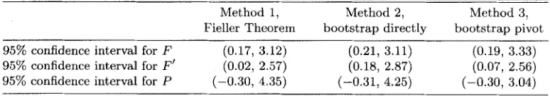
S , Z = O),S = 0 , l . The data in the table suggest that R1, R2, and R3 are true.

Three methods, as described earlier, are used t o construct the confidence intervals for F , F’, and P . The estimated variances of

6

and

6s

from fitted models (1) and (2) are

used as dl1 and $22, and d12 = ~ o r r ( P , B ~ ) ( ~ . 1 1 ~ 2 2 ) ~ ’ ~ , where c 5 r ( B , p s ) is obtained from bootstrap samples. In

this example, the numerator and denominator of F and F’ are functions of the multinomial probabilities, which are asymptotically normal. By the delta method, the variances and covariance for the numerator and denominator of F

(PI)

can be computed. For the bootstrap methods, parametric bootstrapping is used in which 1000 samples are generated from mult inomial distributions.

The resulting 95% confidence intervals for F , F‘, and P estimated from the ophthalmology data are shown in Table 1. Based on the result, the confidence intervals for F and F’ are smaller than the corresponding intervals for P . In the first and second methods, there is at least a 30% reduction in the interval width of F (F’) compared with P. Although the upper bounds of all the confidence intervals are above one, the lower bounds of the confidence intervals for F or F’ are larger than zero, while the lower bounds for P are less than zero. The intervals obtained by the three different methods are fairly close t o each other, which suggests the normal assumption for the numerator and denominator is reasonable. We also observe that there are some differences between the confidence intervals for F and F’ in terms of region covered, with the intervals for F’ shifted t o smaller values.

For a small fraction of the bootstrap samples, the estimates in the denominator of F , F’, or P are close to zero. Of the bootstrapped F

(F’),

1.2% (1%) are outside the range [-4,4] and 2.8% of the bootstrapped P are outside the range [-4,4].

F,

F’,

and P that lie within [-4,4] are plotted against the unadjusted treatment effect

p

(as in model 2) (Figure 2). The plot also suggests that P has a larger variation and that F

and F’ are more likely than P to be concentrated within the range [O, 11.

6. S i m u l a t i o n Study

Simulation studies were carried out to compare the behavior of F and F‘ to P in cases where both T and S are binary. Different sets of data,

{Z

= (0, l ) , S = (0, l), and T = (0, l)}, are generated according to the following two logistic models:

h ^

T a b l e 1

95% Confidence intervals of F , F’, and P for ophthalmology data

Method 1, Method 2, Method 3,

[image:6.612.114.501.663.731.2]

(7)

Use

of

Surrogate Markers

809

[image:7.613.58.301.76.241.2]

-0.5 0.0 0 5 1.0 1 s -0.5 0 0 0.5 1 0 1.5 Unadbted Treatment Elf& Unad&!sled Treatment Enect

Figure 2. Plots of F , F‘, and P from bootstrap samples for ophthalmology data against the unadjusted treatment effect. Only the estimated values that are between [-4,4] are plotted.

(4)

Datasets are created for three scenarios: perfect, useless, and partial surrogates. In each scenario, we simulate 500 datasets and each dataset has a total of 200 subjects randomized t o the treatment group or the placebo group with equal probabilities. The parameter values for each scenario are listed in Table 2. In all simulated cases, conditions Rl-R3 are all satisfied.

We study the bias, variability, and coverage rate of 95% confidence intervals. The true value of F (F’) can be calculated algebraically based on (3) and (4). For P , a large dataset ( n = 2000) is simulated and then logistic models (1) and (2) are fitted on this large dataset t o get the estimate for the true value of P. Ninety-five percent confidence intervals for F , F‘, and P are calculated for each simulated dataset based on Fieller’s Theorem as described earlier.

We show in Table 3 for each scenario the true value of F , F‘, and P , the lower and upper 2.5% percentiles and median of the estimates from 500 datasets, and coverage rate for 95% confidence intervals. The number of times (out of 500) that the 95% confidence intervals for F , F‘, and P lie within [0,1], have lower bounds no smaller than zero, or have upper bounds no larger than one are shown in Table 4.

The results show that the bias for all three estimates are close t o zero. The coverage rates of the 95% confidence intervals based OF Fieller’s Theorem are close to the nominal level. Overall, F and F’ are less variable than P . The ranges of 2.5% and 97.5% percentiles for F and F’ are mostly smaller and are about 30-85% of the ranges for P . In the partial surrogate scenarios, the 2.5% percentiles of

3

and are mostly greater than 0.2, while the 2.5% percentiles of P are mostly below or near zero. Table 4 shows that 95% confidence intervals for F and F’ are, on average, 11 times more likely t o fall between [0, I] than P. In the partial surrogate cases, the number of times that the lower bounds for F and F’ are above zero are 1.5 t o 5.5 times those for P . These results suggest that the variabilities of F and F’ are smaller than P. In the

Table 2

Parameter settings f o r simulations

Scenario cases a1

01

0 2 B.?

Perfect 1 1

.o

3.0 0 0

2 1.5 3.0 0 0

3 1.0 4.0 0 0

Useless 1 0 3.0 0.8 0

2 0 1.5 0.8 0

3 0.5 0 0.8 0

Partial 1 1.0 6.0 0.3 0

2 1.0 3.0 0.45 0

3 1.0 2.0 0.45 0

4 0.5 2.0 0.68 0

5 1.0 2.3 0.68 0.3

6 1.0 2.3 0.68 -0.3

7 1.0 2.3 0.68 0.68

8 1.0 2.3 0.68 -0.68

partial scenarios, which are most likely t o happen in practice, the lower bounds of the confidence intervals for F and F’ are much more likely to be above zero than are the confidence intervals for P , which indicates that F and F’ are more useful

as measures for surrogacy.

Although the variability of F (F’) is smaller than that of P , the results suggest that the confidence intervals for F (F’) are still wide. The majority of the intervals for F and F’ extend beyond zero and/or one, especially the latter, as shown in Ta- ble 4. As discussed earlier, F ( F’ ) are not true proportions with estimates bounded within [0,1]; thus, it is plausible for the values of F and F’ to be outside [0,1]. Table 3 shows that the 2.5% and 97.5% percentiles for F and from the 500 simulated datasets can go outside [0,1], especially on the upper sides. It is not surprising that the confidence intervals can also include values less than zero and greater than one. Freedman (2001) shows that the lengths of the confidence intervals for P using Fieller’s Theorem decrease as the unadjusted treatment effect becomes more significant. For adequate statistical power t o validate surrogate endpoints using P , the unadjusted effect would need t o be five or six times its standard error. It is likely that a stronger treatment effect will also result in shorter confidence intervals for F and F’.

In the partial surrogacy scenarios, as expected, increasing the treatment effect on S and decreasing the treatment effect on T adjusting for S results in larger values for F , F’, and

P.

We observe that P has consistently lower values than F or F‘

inside the interval (0, l), which could be due to the different metrics used in estimating PE.

We also observe that, in the useless surrogate scenarios (cases 1 and 2), where treatment has no effect on the surrogate marker ( a = 0), the large-sample limit for P is negative while the large-sample limit for F and F’ are zero. This suggests that P is not measuring P E appropriately in these situations.

7.

Discussion [image:7.613.312.562.82.282.2] [image:7.613.313.559.83.286.2]

(8)

810

Biometrzcs,

December

2002

Table 3

Results f r o m simulation studies f o r F , F', and P . Shown are the large-sample limit, median of the estimates, upper and lower 2.5% percentiles, and coverage m t e of confidence interval based o n Fieller's Theorem.

Cover age

F F' P

&(2.5%,97.5%)

True value Median

Scenario Cases F F' P F F ' P F F' P

Perfect 1 1 1 1 0.98 0.97 0.96 (0.45, 3.12) (0.47, 3.14) (0.15, 4.86) 0.94 0.95 0.96 2 1 1 1 1.01 0.98 1.00 (0.58, 2.04) (0.58, 1.99) (0.44, 2.68) 0.95 0.95 0.96 3 1 1 1 0.99 0.98 0.94 (0.58, 1.93) (0.58, 2.03) (0.13, 3.48) 0.95 0.95 0.96 Useless 1 0.00 0.00 -0.56 0.00 0.00 -0.54 (-1.84, 1.28) (-1.61, 1.23) (-3.42, 1.31) 0.95 0.98 0.96 2 0.00 0.00 -0.14 0.00 0.00 -0.13 (-0.78, 0.33) (-0.85, 0.35) (-1.16, 0.20) 0.98 0.99 0.94 3 0.00 0.00 0.00 0.00 0.00 -0.00 (-0.24, 0.24) (-0.19, 0.27) (-0.17, 0.18) 0.99 1.0 0.94 Partial 1 0.91 0.85 0.67 0.90 0.84 0.66 (0.64, 1.36) (0.50, 1.49) (-0.24, 2.33) 0.95 0.96 0.95 3 0.54 0.57 0.45 0.54 0.56 0.44 (0.20, 1.52) (0.24, 1.63) (0.06, 1.56) 0.95 0.96 0.95 2 0.71 0.68 0.50 0.69 0.68 0.47 (0.36, 1.32) (0.34, 1.34) (-0.03, 1.60) 0.94 0.96 0.95 4 0.29 0.30 0.11 0.28 0.28 0.10 (-0.10, 0.78) (-0.11, 0.86) (-0.38, 0.79) 0.93 0.98 0.95 5 0.45 0.49 0.27 0.45 0.48 0.25 (0.21, 0.82) (0.23, 0.94) (-0.08, 0.83) 0.95 0.97 0.96 6 0.57 0.52 0.41 0.57 0.50 0.39 (0.26, 1.32) (0.23, 1.25) (0.06, 1.38) 0.95 0.97 0.96 8 0.73 0.55 0.55 0.71 0.55 0.54 (0.27, 2.61) (0.21, 1.92) (0.12, 3.05) 0.95 0.96 0.96 7 0.42 0.48 0.20 0.41 0.48 0.19 (0.20, 0.73) (0.23, 0.87) (-0.15, 0.64) 0.96 0.97 0.96

tion criterion, which requires P(T

I

S , Z ) t o be equal t o P(T

1

S). Freedman et al. (1992) raise the concept of PE in surrogacy validation and propose a quantitative measure of the role a surrogate marker plays in the therapeutic pathways of a treatment. Both of these two approaches focus on the conditional distribution [T

I

S , Z ] in the assessment for surrogate endpoints. Daniels and Hughes (1997) and Buyse et al. (2000) develop a different concept. Let BT denote the treatment effect on the primary endpoint and 0 s the treatment effect on the surrogate marker.

&-

is based on [T

I

21 and is 0 s based on [ S

I

21. In their approaches, the main con- cerns are the relationship between BT and

Bs,

the prediction

of BT based on

Bs,

and the precision of the prediction. The concept of assessing surrogacy by precision of predicting OT

based on the relationship between 0~ and 0 s is a useful one. However, in this approach, the therapeutic pathways through which treatment takes effect is not a major concern as long as the statistical association between OT and 0s is strong. Also, this type of approach is appropriate only if there arc multiple trials available on the same or similar treatments so that the relationship between

OT

and 0 s can be studied.

In this article, we focus on the situation of a single trial and the validation of biomarkers by estimating PE. The underlying motivation for PE comes from thinking of the therapeutic

Table 4

95% Confidence intervals based o n Fieller's Theorem are constructed for each scenario. Shown are the numbers of times ( o u t of 500) that the confidence intervals lie between [O, 11, that lower bounds are

greater than or equal

t o

zero, and that upper bounds are less than or equal to one for F , F ' , and P .

CIS CIS with lower CIS with upper

within [0,1] bound 2 0 bound 51

Scenario Cases F F' P F

F'

P F

F'

P

Perfect 1

2 3

Useless 1

2 3

Partial 1

[image:8.614.58.561.111.308.2] [image:8.614.65.561.524.729.2]

(9)

Use

of

Surrogate Markers

811

pathway. In particular, it is an attempt t o construct a scalar summary that captures the concept that the measure should be one if all of the effect of Z on T is through S, zero if either there is no effect of 2 on S or S is not associated with T , and between zero and one if part of the effect of Z on T is through S . P E is a useful concept for surrogacy validation and F (F’) are proposed as statistical measures for it.

The measure Freedman et al. (1992) proposed has been shown to be problematic. In this article, we propose alternative measures F and F’ and have compared and contrasted them with P . The new measures F and F’ are estimated based on the distributions [S

1

Z ] and [T

1

2, S], which we think is a logical approach because of the temporal relationship between the marker and the primary outcome. F is based on a factor- ization of the joint distribution [T,S

I

21 into [S

I

Z]

and [T

I

S, 21, whereas the measure P is based on consideration of [T

I

S , Z ] and [T

I

21, which together do not necessarily specify the joint distribution [T,S

1

21. I t also seems natural for a measure of surrogacy t o depend directly on how treatment affects the marker. In addition, unlike P , estimation for F is not tied to linear models and can be estimated with more flexibility and fewer assumptions. We think these differences will give F and F” better properties and allow for generalizations. In the case of binary T , our results from the ophthalmology data and the simulation studies suggest that F is less variable than P. In the partial surrogate scenarios, which are most likely to happen in practice, the lower confidence bounds for F and F’ are more likely to be greater than zero than the confidence bounds for P and hence suggests that the new measures are more useful for surrogacy validation.

In cases with repeated measurement of markers, it is often the case that there are dependent censoring or dropouts dur- ing the trial. Fitting model [T

I

21, as required for P , will yield a biased estimate for the treatment effect. However, for F (F’), by joint modeling of [T

I

S,

Z]

and [S

I

Z],

we may reduce the bias in the estimates of treatment effect.

We have proposed two complementary forms of the measure of PE, i.e., F and F‘. An alternative measure based on these two, ( F

+

F‘)/2, can be used. Although population quantities F and F‘ do not equal each other in all situations, ideally, they would be close t o each other. It would be interesting t o further investigate the meaning of the difference between F and F’ in different settings and the properties of their averages.

A drawback for both F ( F’ ) and P is in the interpretation of the estimated values. While values of zero and one have clear interpretations, it is not so easy to understand the exact meaning of an intermediate value. The relative size of F for two different biomarkers in a trial does give an indication of their relative usefulness as a surrogate. The graphical interpretation in Figure 1 is also a useful aid t o the interpretation. We recommend the approach suggested by Freedman et al. (1992) and judge a potential surrogate by whether the lower bound of a confidence interval for F is above a certain value. Although the variability of F (F‘) is smaller than P , the results suggest that the confidence intervals for F (F’) are still wide. The relatively large variability of F (F’), like P , is most likely due t o its inherent limitation as a ratio of estimates. If the denominator is not clearly different from zero, then calculation of the ratio is problematic. It is likely that, for F (F’) t o be useful in validating a surrogate endpoint, a strong treatment effect of

Z

on T would be needed.

In this article, we have focused mainly on the situations of a binary endpoint and a binary surrogate. For future research, extensions of F (F’) to more complex situations will be required. For example, multiple biomarkers or repeated measurements of biomarkers can be considered as the surrogate endpoint. Meta-analysis that combine data across studies may also be used t o increase power and also t o examine the consistency of the underlying proportion F ( F ’ ) across similar studies.

ACKNOWLEDGEMENTS

This work was partially supported by the Early Disease Re- search Network grant CA86400 from the National Cancer In- stitute. The authors thank the editor, the associate editor, and the referees for their helpful suggestions.

RESUMO

Les essais randomisks impliquant des critkres principaux dont l’occurrence est rare, ou dont la mesure est pknaliske par des temps de survenue importants, s’avkrent onkreux. C’est la raison de l’int6ret croissant port6 aux mkthodes consistant a remplacer le veritable critkre clinique par un critbre de substitution, disponible plus pr6cocement. Cependant, ces critkres de substitution doivent 6tre correctement validks. A cet kgard, une mesure quantitative-spkcifique ?i chaque essai-de la

proportion de l’effet traitement expliquke par le crithre de substitution s’avkre un concept utile. Freedman e t al. (1992) ont ainsi suggkrk de mesurer la qualitk de la substitution en calculant le rapport des coefficients de regression associks B l’effet traitement dans deux modkles skparks, ajustks ou non par le critkre de substitution. Cette mesure se rkvhle hklas extrgmement variable, sans compter qu’il n’y a aucune garantie que chacun des deux modhles soit approprik. En nous inspirant d’une id6e formulke par Tsiatis et al. (1995), nous proposons, pour le calcul de cette proportion expliquke, des mkthodes alternatives qui requikrent moins d’hypothbses sous-jacentes au niveau de l’estimation et permettent davan- tage de flexibilitk au niveau de la modklisation. A partir de donnkes issues d’un essai en ophtalmologie, et en utilisant 6galement un certain nombre de simulations, nous comparons les estimations obtenues B l’aide de ces nouvelles mesures, lesquelles semblent de fait prksenter moins de variabilitk.

REFERENCES

Buyse, M. and Molenberghs, G. (1998). Criteria for the validation of surrogate endpoints in randomized experiments. Biometrics 54, 1014-1029.

Buyse, M., Molenberghs, G., Burzykowski, T., Renard, D., and Geys, H. (2000). Validation of surrogate endpoints in meta-analysis of randomized experiments. Biostatistics Bycott, P. W. and Taylor, J. M. G. (1998). An evaluation of a measure of the proportion of the treatment effect explained by a surrogate marker. Controlled Clinical Trials Daniels, M. J. and Hughes, M. D. (1997). Meta-analysis for the evaluation of potential surrogate markers. Statistics in Medicine 16, 1965-1982.

DeGruttola, V., Fleming, T . R., Lin, D. Y . , and Coombs, R.. (1996). Validating surrogate markers: Are we being naive‘? Journal of Infectious Diseuse 175, 237-246. 1, 49-68.

(10)

812

Biometries, December 2002

Efron, B. and Tibshirani, R. (1986). Bootstrap methods for standard errors, confidence intervals, and other measures of statistical accuracy. Statistical Science 1, 54-77. Ellenberg,

S.

S. and Hamilton, J. M. (1989). Surrogate end-

points in clinical trials: Cancer. Statistics i n Medicine 8, Fleming, T. R. (1992). Evaluating therapeutic interventions:

Some issues and experiences. Statistical Science 7, 428- 456.

Fleming, T. R. and DeMets, D. L. (1996). Surrogate endpoints in clinical trials: Are we being misled? Annals of Internal Medicine 125, 605-613.

Freedman,

L.

S. (2001). Confidence intervals and statistical power of the “validation” ratio for surrogate or intermediate endpoints. Journal of Statistical Planning and Inference 96, 143 -153.

Freedman, L. S., Graubard, B. I., and Schatzkin, A . (1992). Statistical validation of intermediate endpoints for chronic disease. Statistics in Medicine 11, 167-

178.

Hwang, G. J. T. (1995). Fieller’s problems and resampling techniques. Statistica Sinica 5 , 161-171.

405-4 13.

Lagakos, S. W. and Hoth, D. F. (1992). Surrogate markers in AIDS: Where are we? Where are we going? Annals of

Internal Medicine 116, 599-601.

Lin, D. Y., Fleming, T. R., and DeGruttola, V. (1997). Esti- mating the proportion of treatment effect explained by a surrogate marker. Statistics in Medicine 16, 1515-1527. Prentice, R. L. (1989). Surrogate endpoints in clinical trials:

Definition and operational criteria. Statistics i n Medicine Schatzkin, A., Freedman, L. S., Schiffman, M. H., and Dawsey, S. M. (1990). Validation of intermediate end points in cancer research. Journal of the National Cancer Institute Tsiatis, A. A., DeGruttola, V., and Wulfsohn, M. S. (1995). Modeling the relationship of survival to longitudinal data measured with error: Applications to survival and CD4

counts in patients with AIDS. Journal of the American Statistical Association 90, 27-37.

8, 431-440.

82, 1746-1752.