R E S E A R C H
Open Access
Convergence of a space-time continuous
Galerkin method for the wave equation
Zhihui Zhao and Hong Li
**Correspondence: [email protected]
School of Mathematical Sciences, Inner Mongolia University, No. 235, West Road of University, Saihan District, Hohhot, 010021, China
Abstract
This paper gives a new theoretical analysis of the space-time continuous Galerkin (STCG) method for the wave equation. We prove the existence and uniqueness of the numerical solutions and get optimal orders of convergence to numerical solutions regarding space that do not need any compatibility conditions on the space and time mesh size. Finally, we employ a numerical example to validate the effectiveness and feasibility of the STCG method.
MSC: 74S10; 65M15; 35Q35
Keywords: continuous Galerkin method; wave equation; optimal orders of convergence; numerical example
1 Introduction
In this article, we analyze the STCG method for the wave equation. As an example, we study the following model of the wave equation: findu=u(x,t) satisfying
⎧ ⎪ ⎨ ⎪ ⎩
utt–u=f(x,t), (x,t)∈×[,T], u(x,t) = , (x,t)∈∂×[,T],
u(x, ) =u(x), ut(x, ) =v(x), x∈,
(.)
whereis a bounded convex polygonal domain in Rwith boundary∂,u
tt=∂u/∂t, ut=∂u/∂t, andT> denotes the total time. The given body forcef and the initial value functionsuandvare sufficiently smooth in order to ensure that the following theoretical analysis is effective.
The STCG method is a kind of finite element technique that uses continuous polynomial functions both in time and space to approximate the evolution problems, that is, it does not only use continuous polynomial functions to discretize space but also uses them to discretize time. Therefore, if we appropriately improve the degrees of polynomials with re-spect to time, we can easily derive any desired order of accuracy. Furthermore, in compar-ison with the theoretical analysis of the classical finite element methods in which the space is discretized by piecewise polynomial functions and the time is discretized by difference quotients, the theoretical analysis of such a method is uniform for any degree polynomials in time used to approximate the time variable. Especially, this method is more effective for solving wave problems since the corresponding discrete schemes retain the energy con-servation properties (see [–]). Owing to the advantages mentioned, it has been applied
extensively to solve various kinds of time-related partial differential equations (TRPDEs) (see,e.g., [–]).
Aziz and Monk [] applied the STCG method to investigate the approximation of the heat equation. French and Peterson [, ] and Bales and Lasiecka [] also studied the ap-proximation of the wave equation through the STCG method. However, the error esti-mates of [] are obtained under the restrictive assumptions that the mesh sizehand time stepkmust satisfyk≤ ˆch, whereˆcis a sufficiently small positive constant. For [, ], al-though the error analysis does not need any compatibility conditions between the space and time mesh size, the theoretical analysis is more abstract and complicated. The main purpose of this article is to propose a new kind of technique to give a theoretical analysis of the STCG method for the wave equation. To achieve this goal, we introduce Legendre polynomials and the corresponding Gauss integration rule and apply the basic properties of Lagrange interpolating polynomials fixed by the Legendre points to prove the existence and uniqueness of the numerical solutions; we also introduce a space-time projection op-erator to analyze the error estimates inLandHnorms between the exact solutions and numerical solutions such that our theoretical analysis is more concise and understandable. Additionally, our error estimates also do not require the time step and space mesh size re-striction. For [, ], the theoretical analysis is starting from an operator equation obtained by the coupled set of equations (.)-(.) by introducing an operator matrix. However, for most of the wave problems, there does not necessarily exist an operator matrix that can be used to make the coupled system become an operator equation. Thus, the theoretical analysis in [, ] have some limitations in some cases. Whereas the analysis showed in this article does not need introducing such an operator matrix, it is directly based on the cou-pled equation set (.)-(.) to study the existence, uniqueness, and convergence of the numerical solution. Therefore, compared with the methods presented in [, ], the idea employed in this paper is relatively easy to be applied to other wave problems. Based on our analysis, we think that the technique used is a kind of improvement and development for the existing papers (see [, , ]).
The rest of this paper is arranged in the following manners. In Section , we give some useful notation and definitions and propose the STCG method for the wave equation. In Section , we complete the error estimates inLandHnorms foruandvwithout any restrictions on the space and time mesh size. In Section , a numerical example is given for illustrating the effectiveness and feasibility of the STCG method. Finally, in Section , we state the main conclusions and some perspectives.
2 STCG method for 2D wave equation
In this article, we use the standard definitions for Sobolev spaces and the corresponding norms (see []). For example, · sand| · |sdenote the usual norms and seminorms of Sobolev spacesHs() (s≥). Whens= , the spaceH() is regarded as the spaceL(), and by (·,·) and · denote the corresponding inner product and norm. Furthermore, we define the energy norm onL()×H() by|(v,u)|={v+∇u}. LetH
() be the subspace ofH() consisting of the functions inH() that vanish on∂. In addition, the spaceHl(,t
n;Hs()) and associated norms are defined by
Hl,tn;Hs()
=
v(x,t); l
j= tn
dtdjjv(·,t)
s dt<∞
and
vHl(,t n;Hs)=
l
j= tn
dtdjjv(·,t)
s dt
/ .
In particular, whenl= ands= , , the associated norms are denoted by
vL(,tn;L)= tn
v(·,t)dt /
and
vL(,t
n;H)=
tn
v(·,t)dt /
,
wheretn(n= , , . . . ,N) are the time nodes of the partition of time interval [,T], which will be defined later. Iftn=T, thenvHl(,tn;Hs)are denoted byvHl(Hs). Noting thatcin
this paper is a general positive constant independent of all discretization parameters but may be different at different places.
Further, if we introduce the functionv=ut, then (.) can be rewritten as the first-order system concerning time
⎧ ⎪ ⎪ ⎪ ⎨ ⎪ ⎪ ⎪ ⎩
vt–u=f, (x,t)∈×[,T], v–ut= , (x,t)∈×[,T], u(x,t) = , (x,t)∈∂×[,T],
u(x, ) =u(x), v(x, ) =v(x), x∈.
(.)
LetU=H(,T;H
()). Then the weak formulation to (.) can be given as follows: find (u,v)∈U×Usatisfying
T
(ut,φt) – (v,φt)
dt= , ∀φ∈U, (.)
T
(vt,ψt) + (∇u,∇ψt)
dt= T
(f,ψt) dt, ∀ψ∈U, (.)
u(x, ) =u, v(x, ) =v, x∈. (.)
In order to formulate the STCG method, let h={K}be a quasi-uniform triangulation partition of discrete regionwithh=maxhK, wherehK stands for the diameter of the triangleK∈ h(see [–]). Then, we introduce the subspaceShm()⊂H() consisting of piecewise continuousmth-degree polynomials defined on the subdivision hofwith mesh parameterh. Let =t<t<· · ·<tN=T be a subdivision on time span [,T] with the maximum time stepk=max≤j≤N|tj–tj–|. LetSkl([,T]) be a finite element space on this subdivision consisting of continuous piecewiselth-degree polynomials regarding time,i.e.,Skl([,T]) ={υ∈C([,T]) :υ|[tj–,tj]∈Pl([tj–,tj]),j= , . . . ,N}, wherePl([tj–,tj])
follows: find (uhk,vhk)∈U
hksuch that T
uhkt ,φt
–vhk,φt
dt= , ∀φ∈Uhk, (.) T
vhk t ,ψt
+∇uhk,∇ψ t
dt=
T
(f,ψt) dt, ∀ψ∈Uhk, (.)
uhk(x, ) =Phu, vhk(x, ) =Phv, x∈. (.)
The STCG solution pair (uhk,vhk) can be computed by marching through successive time levels. To see this, letJn= [tn,tn+], and letPl(Jn) denote the set of polynomials of degreel defined on intervalJn. Then, forn= , , . . . ,N– , we find the STCG solution pair (uhk,vhk) onJnsatisfying
Jn
uhkt ,φt
–vhk,φt
dt= , ∀φ∈Shm()⊗Pl(Jn), (.)
Jn
vhkt ,ψt
+∇uhk,∇ψt
dt=
Jn
(f,ψt) dt, ∀ψ∈Shm()⊗Pl(Jn) (.)
or, equivalently,
Jn
uhkt ,φ–vhk,φdt= , ∀φ∈Shm()⊗Pl–(Jn), (.)
Jn
vhkt ,ψ+∇uhk,∇ψdt
=
Jn
(f,ψ) dt, ∀ψ∈Shm()⊗Pl–(Jn), (.)
withuhk(x, ) =P
hu,vhk(x, ) =Phv(wherePhis the elliptic projection defined further in (.)), anduhk(x,t
n),vhk(x,tn) (n= , , . . . ,N– ,x∈) have been fixed at previous time level.
Remark In fact, (.)-(.) can be regarded as the Petrov-Galerkin method since they are tested byφtandψt, respectively.
To analyze the well-posedness of problem (.)-(.), we need to introduce the Legen-dre polynomials and the corresponding Gauss integration rule. For a givenl≥, let{i}li= be the Lagrange interpolating polynomials of degreel– , that is,
i(μ) = l
j=,j=i
(μ–μj) (μi–μj)
, (.)
where the interpolating points <μ<· · ·<μl< arelroots of the Legendre polynomial on the interval [, ]. Then the Gauss-Legendre integration formula is as follows:
m(μ) dμ∼= l
j=
ωjm(μj), (.)
whereωj=
Further, applying the linear transformationt=tn+μkn(kn=tn+–tn) that maps the unit interval [, ] onto the intervalJn, its quadrature points and weights are defined by
⎧ ⎪ ⎨ ⎪ ⎩
tn,i=tn+μikn, i= , . . . ,l,
n,i(t) =i(μ),
ωn,i= tn+
tn n,i(t) dt=kn
i(μ) dμ=knωi, i= , . . . ,l.
(.)
Then the Gauss-Legendre integration formula associated withJnis as follows:
tn+
tn
m(t) dt∼= l
i=
ωn,im(tn,i). (.)
We also need to employ the Lagrange interpolating polynomials{ ˜i}li=of degreel corre-sponding to thel+ interpolating points =μ<μ<· · ·<μl< , that is,
˜
i(μ) = l
j=,j=i
(μ–μj) (μi–μj) .
Choosing{ ˜n,i}li= (where˜n,i(t) =˜i(μ)) as the basis functions to the polynomial space Pl(Jn), then (uhk,vhk)|Jnare solely fixed by the functions (uhkn,i,vnhk,i) = (uhk(x,tn.i),vhk(x,tn.i))∈ Shm×Shmsuch that
uhk(x,t) = l
i= ˜
n,i(t)uhkn,i(x), vhk(x,t) = l
i= ˜
n,i(t)vhkn,i(x), (x,t)∈×Jn,
wheretn,=tn.
Further, let (uhkn,i,vnhk,i) = (u˜hkn,iμ/i ,v˜hkn,iμ/i ) (i= , . . . ,l). Then the new expressions for uhk(x,t) andvhk(x,t) can be rewritten as
uhk(x,t) = l
i= ˜
n,i(t)uhkn,i(x)
= l
i=
μ/i ˜n,i(t)u˜hkn,i(x) +˜n,(t)uhkn,(x), (.)
vhk(x,t) = l
i= ˜
n,i(t)vhkn,i(x)
= l
i=
μ/i ˜n,i(t)˜vhkn,i(x) +˜n,(t)vhkn,(x). (.)
By choosing (φ,ψ) = (μ–/i n,iϕ,μ–/i n,iϕ) (whereϕi∈Shm,i= , ) in (.) and (.) we can equivalently rewrite the STCG scheme (.)-(.) for (u˜hkn,j,v˜hkn,j) (j= , , . . . ,l) as
⎧ ⎪ ⎨ ⎪ ⎩
l
j=b˜ij(˜uhkn,j,ϕ) –knωi(˜vhkn,i,ϕ) = –μi–/bi(uhkn,,ϕ), l
j=b˜ij(˜vhkn,j,ϕ) +knωi(∇ ˜uhkn,i,∇ϕ) = –μ–/i bi(vhkn,,ϕ) +
Jnμ
–/
i n,i(f,ϕ) dt, i= , . . . ,l,
where
˜
bij=μ–/i bijμ/j , bij=
Jn
˜
n,j(t)n,i(t) dt, i= , . . . ,l,j= , , . . . ,l. (.)
Remark To illustrate how to use (.) to solve the numerical solution, we takel= for example. In this case,˜n,j(t) (j= , , ) is determined viatn,,tn,, andtn,or via (.), which is equivalently fixed by ,μ, andμ, andn,i(i= , ) is fixed viatn,,tn,(orμ,μ), whereμ,μare the two roots of the quadratic Lengendre polynomial defined in interval [, ]. Therefore, by (.) we can obtain the values ofb˜ij(i,j= , ) andbi(i= , ). In addition, sinceu˜hk
n,jandv˜hkn,jare elements ofShm, they can be expressed as follows:
˜
uhkn,j=cj,χ+cj,χ+· · ·+cj,nχn,
˜
vhkn,j=dj,χ+dj,χ+· · ·+dj,nχn,
(.)
where χi (i= , , . . . ,n) denote the basis functions ofShm, andnstands for the dimen-sion ofShm. Then we substitute (.) into (.) and letϕandϕtakeχi(i= , , . . . ,n), respectively. We finally obtain the set of equations
⎛ ⎜ ⎜ ⎜ ⎝
knωA –bA˜ –bA˜ knωA –bA˜ –bA˜ ˜
bA bA˜ knωM ˜
bA bA˜ knωM ⎞ ⎟ ⎟ ⎟ ⎠
⎛ ⎜ ⎜ ⎜ ⎝
d d c c
⎞ ⎟ ⎟ ⎟ ⎠=
⎛ ⎜ ⎜ ⎜ ⎝ f f g g
⎞ ⎟ ⎟ ⎟
⎠, (.)
where A= (aij)n×n, aij= (χi,χj), M= (mij)n×n, mij= (∇χi,∇χj). ci= (ci,,ci,, . . . ,ci,n)T, di= (di,,di,, . . . ,di,n)T (i= , ).fi= (fi,,fi,, . . . ,fi,n)T,gi= (gi,,gi,, . . . ,gi,n)T (i= , ),fi,j= –μ–/i bi(uhkn,,χj),gi,j= –μ–/i bi(vhkn,,χj) +
Jnμ
–/
i n,i(f,χj) dt(j= , , . . . ,n). We notice that uhkn, andvhkn, have been found in the previous time level. Therefore, by (.) and (.), (.) we can obtainuhk(x,t) andvhk(x,t).
Furthermore, the following lemma holds (see []).
Lemma Letλ:=
minj
ωj μj.Then
xTBx ≥λ|x|=λ
l
i= xi
, ∀x∈Rl, (.)
whereB=D–/BD/,B= (bij)l×l,and D=diag{μ, . . . ,μl}.
For further theoretical analysis, we need to introduce the discrete operatorAh:L()→ Shm() defined by
(∇Ahu,∇φ) = (u,φ), ∀φ∈Shm(). (.)
From this definition we can easily prove thatAh is a nonnegative self-adjoint operator. Therefore, there exists a square-root operatorA/h satisfying (u,Ahu) = (A/h u,A/h u) (∀u∈ L()). Furthermore,A
Shm, then (φ,φ) = (∇Ahφ,∇φ) = , that is,φ= . Note thatAh can also be extended to functions inL(,T;L()) in theLsense.
Theorem Assume that the solution pair(uhk(t
n),vhk(tn))is given in the time level Jn–. Then,for k small enough,there exists a unique solution pair(uhk,vhk)∈(S
hm()⊗Pl(Jn)) to the system of equation(.)-(.).
Proof Since (.)-(.) is a linear system of equations, in order to demonstrate the exis-tence and uniqueness of its approximate solutions, we only need to prove that iff = and uhkn,=vhkn,= , then there is a zero solution pair to it.
Taking (ϕ,ϕ) = (u˜hkn,i,Ahv˜hkn,i) in (.), we have
l
i,j= ˜ bij
˜
uhkn,j,u˜hkn,i+Ah/v˜hkn,j,A/h v˜hkn,i
= – l
i=
μ–/i bi
uhk n,,u˜hkn,i
+A/h vhk
n,,A/h v˜hkn,i
+ l
i=
Jn
μ–/i n,i
Ah/f,A/h v˜hkn,idt. (.)
For the terms of the left side of (.), in view of Lemma , we have
λ
l
i= u˜hk
n,i
+A/h ˜vhkn,i≤ l
i,j= ˜ bij
˜
uhkn,j,u˜nhk,i+A/h v˜hkn,j,A/h ˜vhkn,i . (.)
For the first part of the right side of (.), using the Hölder and Cauchy inequalities, we have
l
i=
μ–/i bi
uhk n,,u˜hkn,i
+A/
h vhkn,,A/h v˜hkn,i
≤ l
i=
μ–/i
˜
(μ)i(μ) dμunhk,u˜hkn,i+A/h v hk
n,A/h u˜ hk n,i
≤ c λ
l
i=
uhkn,+A/h vhkn,+λ
l
i=
u˜hkn,i+A/h v˜hkn,i. (.)
Also, by the Hölder and Cauchy inequalities, noting thatJ
n
n,i(t) dt=knωi, for the second part of the right side of (.), we derive
l
i=
Jn
μ–/i n,i
A/h f,A/h v˜hkn,idt
≤cA/h fL(J
n;L)+ck
l
i= A/
h v˜hkn,i
Combining (.) with (.)-(.) and assuming thatk≤λc, we have
λ
l
i= u˜hk
n,i
+A/h v˜hkn,i
≤λ
l
i= u˜hk
n,i
+ !
λ
–ck " l
i=
A/h v˜hk n,i
≤ c λ
l
i=
uhkn,+A/h vhkn,+cA/h fL(J
n;L). (.)
Settingf = anduhkn,=vhkn,= in (.), sinceA/h invertible onShm, we getu˜hkn,i=v˜hkn,i= (i= , , . . . ,l), that is,uhk=vhk= . Because the existence of the solution is implied by the uniqueness, system (.)-(.) has a unique solution pair.
3 Error estimates of the STCG solutions
In this section, we give some error estimates between the approximate solutions and exact solutions. To this end, we need to introduce some projections.
We define the space variable Ritz projectionPh:H()→Shm(), that is, foru∈H(), we have
(∇Phu,∇φh) = (∇u,∇φh), ∀φh∈Shm(). (.)
Because of the regularity of the triangulation h, we know thatPh has the following ap-proximation properties (see [, ]). Ifu∈H()∩Hs(), then
Phu–ur≤chs–rus, ≤s≤m+ ;r= , . (.)
The projectionPhcan be generalized to functions oftandxin theLsense. Namely, we define the generalized projectionPh:L(,T;H())→Shm()×L(,T) by
T
(∇Phu,∇φh) dt= T
(∇u,∇φh) dt, ∀φ∈Shm()⊗L(,T). (.)
Furthermore, we need to define the time projectionPk :H(,T)→Skl([,T]) as well; namely, forw∈H(,T), it satisfiesPkw() =w() and
T
(Pkw)tφktdt= T
wtφtkdt, ∀φk∈Skl
[,T]. (.)
We can easily conclude from the classical FE techniques thatPk satisfies the following estimate: forw∈H(,T)∩Hs(,T),
Pkw–wHr(,T)≤chs–rwHs(,T), –l+ ≤r≤≤s≤l+ . (.)
Also, we can generalizePkto functions oftandxin theLsense. Thus, we definePk: H(,T;L())→L()×Skl([,T]) by
T
(Pkw)t,φtk
dt= T
wt,φtk
dt, ∀φk∈L()⊗Skl
with initial condition (Pkw(),φ) = (w(),φ) (∀φ∈L()). Further, from (.) we conclude that Pkw(tn) =w(tn) (n= , , , . . . ,N). Moreover, the projectionsPh andPk satisfy the following properties (see []).
Lemma Let Phand Pkbe defined in the generalized sense via(.)and(.).
() Letv∈H(,T;H()).Then
(Phv)t=Phvt, ∇(Pkv) =Pk∇v,
PhPkv=PkPhv, AhPkv=PkAhv.
(.)
() Letv∈Hs(,t
n;L()).Then,for–l+ ≤r≤≤s≤l+ ,
n–
m=
v–PkvHr(J
m)dx≤ck
(s–r)v
Hs(,tn;L). (.)
() Letv∈H(,T;Hm+())∩H(,T;H
())for allt∈[,T].Then
(v–Phv)(t)r≤chm+–rv(t)m+, r= , . (.)
() Letv∈L(,t
n;Hs())∩H(,tn;H()).Then
(v–Phv)(t)L(,tn;L)≤chsv(t)L(,tn;Hs), ≤s≤m+ . (.)
() Letv∈Hl+(,t
n;L())∩H(,tn;H())and vt∈L(,tn;Hm+())∩H(,tn;H()).Then
(v–PhPkv)tL(,t
n;L)≤c
hm+vtL(,tn;Hm+)+klvHl+(,t
n;L) . (.)
Lemma Let Ph and Pkbe the projections defined before,and let u,v∈H(,tn;H()).
Then,for any(ψ,φ)∈Uhk ,we have
tn
Phv–vhk
t,ψt
+∇PkPhu–uhk
,∇ψt
dt
= tn
(Phv–v)t,ψt
+∇(Pku–u),∇ψt
dt (.)
and tn
PkPhu–uhk
t,φt
–Phv–vhk,φt
dt= . (.)
Proof From the definitions ofPhandPkand the properties of the projections we get
tn
Phv–vhk
t,ψt
+∇PkPhu–uhk
,∇ψt
dt
= tn
(Phv–v)t,ψt
+∇(PkPhu–Phu),∇ψt
+ tn
v–vhkt,ψt
+∇Phu–uhk
,∇ψt
dt
= tn
(Phv–v)t,ψt
+∇(Pku–u),∇ψt
dt
+ tn
v–vhkt,ψt
+∇u–uhk,∇ψt
dt. (.)
In addition,
tn
PkPhu–uhk
t,φt
–Phv–vhk
,φt
dt
= tn
(PkPhu–u)t,φt
– (Phv–v,φt)
dt
+ tn
u–uhkt,φt
–v–vhk,φt
dt
= tn
(Phu–u)t,φt
– (Phv–v,φt)
dt
+ tn
u–uhkt,φt
–v–vhk,φt
dt. (.)
Because (u,v) and (uhk,vhk) are solution pairs of (.)-(.) and (.)-(.), respectively, combining (.)-(.) with the factv=ut finishes the proof of Lemma .
In order to continue the theoretical analysis, the following Gronwall lemma needs to be recalled. In the sequel, it will be used frequently.
Lemma (Gronwall Lemma) Suppose y(s),g(s),h(s)are three nonnegative locally inte-grable functions on the interval[,∞)and that,for any given tand all t≥t,the following inequality holds:
g(t) +W(t)≤C+ t
t
y(τ) dτ+ t
t
g(τ)h(τ) dτ. (.)
Then,
g(t) +W(t)≤ !
C+ t
t y(τ) dτ
"
exp
! t
t h(τ) dτ
"
, (.)
where W(t)is a nonnegative function,and C≥represents a positive constant that does not depend on k and h.
The results on the convergence of the numerical solutions of (.)-(.) are given in the following theorems and corollary.
Theorem Let(u(x,t),v(x,t))be a solution pair of(.)-(.),and let(uhk(x,t),vhk(x,t))
() Let∇u∈Hm+()for≤t≤T,u∈Hl+(,T;L()),v
t∈H(,T;Hm+()),
andvtt∈L(,T;Hm+()).Then u(tn) –uhk(tn)
≤C #
hm$∇u(tn)m++vttL(,t
n;Hm+)+ sup
≤t≤tn
vtm+ %
+kluHl+(,tn;L) &
, n= , , . . . ,N. (.)
() Letv∈Hm+()for≤t≤T,u∈Hl+(,T;L()),v
t∈H(,T;Hm+()),and vtt∈L(,T;Hm+()).Then
v(tn) –vhk(tn)
≤C#hm+$v(tn)m++vttL(,tn;Hm+)+ sup ≤t≤tn
vtm+ %
+kluHl+(,t
n;L)
&
, n= , , . . . ,N. (.)
Proof Taking (ψ,φ) = (PkPhu–uhk,Phv–vhk) in (.) and (.), we obtain tn
Phv–vhk,
Phv–vhk
t
+∇PkPhu–uhk
,∇PkPhu–uhk t dt = tn
(Phv–v)t,
PkPhu–uhk
t
+(Pku–u),
PkPhu–uhk
t
dt. (.)
Noting that (Phv(),Phu()) = (vhk(),uhk()) andPkw(tn) =w(tn) (∀w∈H(,T)) and us-ing integration by parts to the right side of (.), we have
Phv(tn) –v hk(t n) + ∇
PhPku(tn) –uhk(tn)
≤(Phv–v)t(tn),
PkPhu–uhk
(tn)
+ tn
PkPhu–uhk, (Phv–v)tt dt + tn
PkPhu–uhk,(Pku–u)t
dt. (.)
Using the Hölder and Cauchy inequalities, we have Phv(tn) –vhk(tn)+∇
PhPku(tn) –uhk(tn)
≤c(Phv–v)t(tn)
+c tn
(Phv–v)tt
dt
+c tn
(Pku–u)t
dt+ tn
∇
PkPhu–uhkdt. (.)
Applying the Gronwall lemma to (.) yields Phv(tn) –vhk(tn)
+∇
PhPku(tn) –uhk(tn)
≤c max
≤t≤T
(Phv–v)t+c tn
(Phv–v)ttdt+c tn
By the triangle inequality and (.), noting thatPkPhu(tn) =Phu(tn), we see that
∇
u(tn) –uhk(tn)≤∇
u(tn) –Phu(tn)+∇
PkPhu(tn) –uhk(tn) ≤c sup
≤t≤T
(Phv–v)t+c(Phv–v)tt L(,t
n;L)
+c(Pku–u)tL(,tn;L)+∇
u(tn) –Phu(tn). (.)
Then (.) follows from (.) and Lemma . Again, using the triangle inequality and (.), we obtain
v(tn) –vhk(tn)≤v(tn) –Phv(tn)+Phv(tn) –vhk(tn) ≤c sup
≤t≤T
(Phv–v)t+c(Phv–v)ttL(,t
n;L)
+c(Pku–u)tL(,tn;L)+v(tn) –Phv(tn). (.)
By (.) and Lemma we finish the proof of part of Theorem .
We also give the energy norm estimate in the following corollary.
Corollary Suppose that the conditions of the Theoremhold.Then
u(tn) –uhk(tn)+v(tn) –vhk(tn)
≤C #
hm$∇u(tn)m++v(tn)m++vttL(,tn;Hm+)+ sup ≤t≤tn
vtm+ %
+kluHl+(,tn;L) &
, n= , , . . . ,N. (.)
Proof The corollary is directly demonstrated via the results (.) and (.) of
Theo-rem .
Theorem Suppose that solutions u and v to (.)-(.) are smooth enough so that
u∈ Hm+() for ≤t≤T, u∈Hl+(,T;L()), vt ∈H(,T;Hm+()), and vtt ∈ L(,T;Hm+()).Then we have
u(tn) –uhk(tn)≤C #
hm+$u(tn)m++vttL(,tn;Hm+)+ sup ≤t≤T
vtm+ %
+kluHl+(,t
n;L)
&
, n= , , . . . ,N. (.)
Proof Setting (ψ,ϕ) = (Ah(PkPhu–uhk),Ah(Phv–vhk)) in (.) and (.) and applying the definition and symmetry property ofAh, we obtain
tn
Phv–vhk
,Ah
Phv–vhk
t
+PkPhu–uhk
,PkPhu–uhk
t
dt
= tn
(Phv–v)t,Ah
PkPhu–uhk
t
dt
+ tn
∇(Pku–u),∇Ah
PkPhu–uhk
t
From the initial condition (Phv(),Phu()) = (vhk(),uhk()) and Pkw(tn) =w(tn) (∀w∈ H(,T)), using integration by parts to the right side of (.), we see that
A
/ h
Phv–vhk
(tn) +
PkPhu–u hk(t
n)
≤Ah(Phv–v)t(tn),
PkPhu–uhk
(tn)
+ tn
PkPhu–uhk,Ah(Phv–v)tt
dt
+ tn
PkPhu–uhk,Ah(Pku–u)t
dt. (.)
Further, using the Hölder and Cauchy inequalities, we have that
A/h Phv–vhk
(tn)+PkPhu(tn) –uhk(tn)
≤c sup
≤t≤T
Ah(Phv–v)t+c tn
Ah(Phv–v)ttdt
+c tn
Ah(Pku–u)t
dt+ tn
PkPhu–uhk
dt. (.)
Applying the Gronwall lemma to (.) yields
A/h Phv–vhk
(tn)
+PkPhu(tn) –uhk(tn)
≤c sup
≤t≤T
Ah(Phv–v)t+c tn
Ah(Phv–v)ttdt
+c tn
Ah(u–Pku)tdt. (.)
Therefore, applying the triangle inequality to (.), we get that
u(tn) –uhk(tn)
≤u(tn) –Phu(tn)+PkPhu(tn) –uhk(tn) ≤c sup
≤t≤T
Ah(Phv–v)t+cAh(Phv–v)ttL(,t
n;L)
+cAh(Pku–u)tL(,t
n;L)+u(tn) –Phu(tn). (.)
Inequality (.) now directly follows from (.), the boundedness ofAh, and Lemma .
Theorem Let ∇v∈ Hm+() for ≤ t ≤T, u ∈ Hl+(,T;L()), v
t ∈ H(,T; Hm+()),and v
tt∈L(,T;Hm+()).Then
v(tn) –vhk(tn)≤C #
hm$∇v(tn)m++vttL(,tn;Hm+)+ sup ≤t≤tn
vtm+ %
+kluHl+(,t
n;L)
&
Proof We first introduce the discrete space-time operatorTh:L(,T;H())→Shm()× L(,T) satisfying
T
(Thχ,φ) dt= T
(∇χ,∇φ) dt, ∀φ∈Shm()×L(,T). (.)
Taking (ψ,ϕ) = (Th(PkPhu–uhk),Th(Phv–vhk)) in (.) and (.) and applying the definition ofTh, we obtain
tn
∇Phv–vhk
,∇Phv–vhk
t
+Th
PkPhu–uhk
,Th
PkPhu–uhk t dt = tn
(Phv–v)t,Th
PkPhu–uhk t dt – tn
(Pku–u),Th
PkPhu–uhk t dt. (.) Further, ∇
Phv–vhk
(tn)
+Th
PkPhu–uhk
(tn)
≤c sup
≤t≤T
(Phv–v)t
+c tn
(Phv–v)tt
dt
+c tn
(Pku–u)t
dt+ tn
Th
PkPhu–uhk
dt. (.)
Then applying the Gronwall lemma to (.) yields
∇
Phv–vhk
(tn)
+Th
PkPhu–uhk
(tn)
≤c sup
≤t≤T
(Phv–v)t
+c tn
(Phv–v)tt
dt
+c tn
(Pku–u)tdt. (.)
Therefore,
∇
v–vhk(tn)
≤∇(v–Phv)(tn)+∇
Phv–vhk
(tn) ≤c sup
≤t≤T
(Phv–v)t+c(Phv–v)ttL(,tn;L)
+c(Pku–u)tL(,tn;L)+∇(v–Phv)(tn). (.)
In view of (.), Lemma completes the proof for Theorem .
4 Numerical example
Figure 1 A partition of the domain withh= 1/16.
Table 1 The errors and convergence rates ofu–uhkin theL2andH1norms concerninghat t= 1
h Error inL2 Rate Error inH1 Rate
1/8 4.8975e–2 1.6055e–0
1/16 1.2272e–2 1.9967 8.0820e–1 0.9902 1/32 3.0747e–3 1.9968 4.0534e–1 0.9956 1/64 7.6265e–4 2.0113 2.0206e–2 1.0043
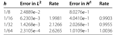
Table 2 The errors and convergence rates ofv–vhkin theL2andH1norms concerninghat t= 1
h Error inL2 Rate Error inH1 Rate
1/8 2.4889e–2 8.0276e–1
1/16 6.2303e–3 1.9981 4.0410e–1 0.9903 1/32 1.4268e–3 2.1266 2.0268e–1 0.9955 1/64 2.3105e–4 2.6265 1.0109e–1 1.0036
Table 3 The errors and convergence rates ofu–uhkin theL2(L2) andL2(H1) norms concerningh
h Error inL2(L2) Rate Error inL2(H1) Rate
1/8 6.4243e–2 2.1045e–0
1/16 1.6078e–2 1.9985 1.0594e–0 0.9902 1/32 4.0188e–3 2.0003 5.3134e–1 0.9956 1/64 9.8849e–4 2.0235 2.6487e–1 1.0043
= [, ]and the time spanI= [, ]. The exact solutionsu=e–tsin(πx)sin(πy) and v= –e–tsin(πx)sin(πy) are established by (.) iff= ( + π)e–tsin(πx)sin(πy), u =sin(πx)sin(πy), and v = –sin(πx)sin(πy). We set discrete initial values (uhk(),vhk()) = (P
hu,Phv). We also provide the errors and orders of convergence in theL(L) andL(H) norms foru–uhk andv–vhkconcerninghandk. All the experi-ments are simulated on unstructured meshes (see Figure ) and computed fromt= to t= .
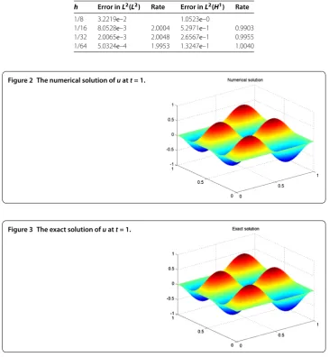
[image:15.595.204.386.368.424.2] [image:15.595.196.397.472.529.2]Table 4 The errors and convergence rates ofv–vhkin theL2(L2) andL2(H1) norms concerningh
h Error inL2(L2) Rate Error inL2(H1) Rate
1/8 3.2219e–2 1.0523e–0
[image:16.595.115.481.109.506.2]1/16 8.0528e–3 2.0004 5.2971e–1 0.9903 1/32 2.0065e–3 2.0048 2.6567e–1 0.9955 1/64 5.0324e–4 1.9953 1.3247e–1 1.0040
Figure 2 The numerical solution ofuatt= 1.
Figure 3 The exact solution ofuatt= 1.
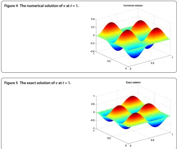
provide the plots to numerical solutions and exact solutions foruin Figure and Figure and forvin Figure and Figure withh= /, both of which show that the numerical solutions are very close to the exact solutions.
Next, we analyze the orders of convergence with respect tok. Because we takel= in this example, the errors in theL(L),L(H),L, andHnorms theoretically should have the third-order accuracy concerningk. Thus, in order to study the orders of convergence in theL∞(L),LandL∞(H),Hnorms concerningk, we takeh=O(k/) andh=O(k), respectively. In this case, the errors are only functions of time stepk. Table , Table , Table , and Table show that the orders of convergence foru–uhkandv–vhk in these norms near third-order accuracy concerningk, respectively, which are one order accuracy higher than the theoretical findings.
5 Conclusions and perspectives
Figure 4 The numerical solution ofvatt= 1.
[image:17.595.160.427.424.471.2]Figure 5 The exact solution ofvatt= 1.
Table 5 The errors and convergence rates ofu–uhkin theL2andH1norms concerningkat t= 1
(h, k) Error inL2 Rate (h, k) Error inH1 Rate
(0.125, 1/4) 2.4620e–2 (1/8, 1/2) 8.0728e–1
[image:17.595.167.426.511.557.2](0.0442, 1/8) 3.1414e–3 2.9703 (1/27, 1/3) 2.4231e–1 2.9681 (0.0156, 1/16) 3.9093e–4 3.0064 (1/64, 1/4) 1.0114e–1 3.0372
Table 6 The errors and convergence rates ofv–vhkin theL2andH1norms concerningkat t= 1
(h, k) Error inL2 Rate (h, k) Error inH1 Rate
(0.125, 1/4) 1.2556e–2 (1/8, 1/2) 4.0417e–1
[image:17.595.155.439.597.645.2](0.0442, 1/8) 1.5500e–3 3.0181 (1/27, 1/3) 1.2116e–1 2.9712 (0.0156, 1/16) 1.1918e–4 3.7010 (1/64, 1/4) 5.0577e–2 3.0367
Table 7 The errors and convergence rates ofu–uhkin theL2(L2) andL2(H1) norms concerningk
(h, k) Error inL2(L2) Rate (h, k) Error inL2(H1) Rate
(0.125, 1/4) 3.2246e–2 (1/8, 1/2) 1.0582e–0
[image:17.595.154.440.686.732.2](0.0442, 1/8) 4.1121e–3 2.9712 (1/27, 1/3) 3.1763e–1 2.9681 (0.0156, 1/16) 5.0685e–4 3.0203 (1/64, 1/4) 1.3257e–1 3.0372
Table 8 The errors and convergence rates ofv–vhkin theL2(L2) andL2(H1) norms
concerningk
(h, k) Error inL2(L2) Rate (h, k) Error inL2(H1) Rate
(0.125, 1/4) 1.6141e–2 (1/8, 1/2) 5.2912e–1
error estimates in theLandHnorms foruandvregarding space. The theoretical anal-ysis presented in this paper is different from those in [, , ] since we introduce Legendre polynomials and the corresponding Gauss integration rule to study the well-posedness of the STCG scheme and introduce a space-time projection operator to analyze the error estimates in theLandHnorms foru–uhkandv–vhksuch that our theoretical analysis is more concise and understandable. Especially, our techniques can be easily extended to other TRPDEs. Thus, we develop and improve the existing results. Finally, a numerical ex-ample is given to validate the feasibility and efficiency of the STCG method. In the future work, we hope that the approach used in this paper will be a foundation for the nonlinear problems, such as the KdV equation, the Klein-Gordon equation, and so on. Moveover, although the STCG method can easily improve the accuracy of approximate solutions, it has lots of degrees of freedom; so in the forthcoming work, we plan to investigate the reduced-order STCG method based on a proper orthogonal decomposition for the wave equation.
Competing interests
The authors declare that they have no competing interests.
Authors’ contributions
Both authors contributed equally and significantly in writing this article. All authors read and approved the final manuscript.
Acknowledgements
This research was supported by National Science Foundation of China grant (11361035, 11271127, 11301258), Natural Science Foundation of Inner Mongolia (2014BS0101), Postgraduate Scientific Research Innovation Foundation of Inner Mongolia (11200-12110201).
Received: 3 July 2016 Accepted: 21 October 2016 References
1. French, DA, Schaeffer, JW: Continuous finite element methods which preserve energy properties for nonlinear problems. Appl. Math. Comput.39, 271-295 (1991)
2. Glassey, RT: Convergence of an energy preserving scheme for the Zakharov equations in one space dimension. Math. Comput.58, 83-102 (1992)
3. French, DA, Peterson, TE: A continuous space-time finite element method for the wave equation. Math. Comput. 65(214), 491-506 (1996)
4. Aziz, AK, Monk, P: Continuous finite elements in space and time for the heat equation. Math. Comput.52, 255-274 (1989)
5. Bales, L, Lasiecka, I: Negative norm estimates for fully discrete finite element approximates to the wave equation with nonhomogeneousL2Dirichlet boundary data. Math. Comput.64, 89-115 (1995)
6. Li, H, Zhao, ZH, Luo, ZD: A space-time continuous finite element method for 2D viscoelastic wave equation. Bound. Value Probl. (2016). doi:10.1186/s13661-016-0563-1
7. Zhao, ZH, Li, H, Luo, ZD: A new space-time continuous Galerkin method with mesh modification for Sobolev equations. J. Math. Anal. Appl.440, 86-105 (2016)
8. French, DA: A space-time finite element method for the wave equation. Comput. Methods Appl. Mech. Eng.107, 145-157 (1993)
9. Bales, L, Lasiecka, I: Continuous finite elements in space and time for the nonhomogeneous wave equation. Comput. Math. Appl.27(3), 91-102 (1994)
10. Adams, RA: Sobolev Spaces. Academic Press, New York (1975)
11. Luo, ZD: The Foundations and Applications of Mixed Finite Element Methods. Chinese Science Press, Beijing (2006) (in Chinese)
12. Brezzi, F, Fortin, M: Mixed and Hybrid Finite Element Methods. Springer, New York (1991) 13. Ciarlet, PG: The Finite Element Method for Elliptic Problems. North-Holland, Amsterdam (1978)