Volume 2010, Article ID 657192,20pages doi:10.1155/2010/657192
Research Article
A New Method for Solving Monotone Generalized
Variational Inequalities
Pham Ngoc Anh and Jong Kyu Kim
Department of Mathematics, Kyungnam University, Masan, Kyungnam 631-701, Republic of Korea
Correspondence should be addressed to Jong Kyu Kim,[email protected] Received 11 May 2010; Revised 27 August 2010; Accepted 4 October 2010
Academic Editor: Siegfried Carl
Copyrightq2010 P. N. Anh and J. K. Kim. This is an open access article distributed under the Creative Commons Attribution License, which permits unrestricted use, distribution, and reproduction in any medium, provided the original work is properly cited.
We suggest new dual algorithms and iterative methods for solving monotone generalized variational inequalities. Instead of working on the primal space, this method performs a dual step on the dual space by using the dual gap function. Under the suitable conditions, we prove the convergence of the proposed algorithms and estimate their complexity to reach anε-solution. Some preliminary computational results are reported.
1. Introduction
LetCbe a convex subset of the real Euclidean spaceRn,F be a continuous mapping fromC intoRn, andϕbe a lower semicontinuous convex function fromCintoR. We say that a point
x∗is a solution of the following generalized variational inequality if it satisfies
Fx∗, x−x∗ϕx−ϕx∗≥0, ∀x∈C, GVI
where·,·denotes the standard dot product inRn.
Associated with the problemGVI, the dual form of this is expressed as following which is to findy∗∈Csuch that
Fx, x−y∗ϕx−ϕy∗≥0, ∀x∈C. DGVI
It is well known that the interior quadratic and dual technique are powerfull tools for analyzing and solving the optimization problems see10–16. Recently these techniques have been used to develop proximal iterative algorithm for variational inequalitiessee17– 22.
In addition Nesterov 23 introduced a dual extrapolation method for solving variational inequalities. Instead of working on the primal space, this method performs a dual step on the dual space.
In this paper we extend results in 23 to the generalized variational inequality problemGVIin the dual space. In the first approach, a gap functiongxis constructed such thatgx ≥ 0, for allx∗ ∈ Candgx∗ 0 if and only ifx∗solvesGVI. Namely, we first develop a convergent algorithm forGVIwithFbeing monotone function satisfying a certain Lipschitz type condition onC. Next, in order to avoid the Lipschitz condition we will show how to find a regularization parameter at every iterationksuch that the sequencexk converges to a solution ofGVI.
The remaining part of the paper is organized as follows. In Section 2, we present two convergent algorithms for monotone and generalized variational inequality problems with Lipschitzian condition and without Lipschitzian condition.Section 3deals with some preliminary results of the proposed methods.
2. Preliminaries
First, let us recall the well-known concepts of monotonicity that will be used in the sequel
see24.
Definition 2.1. LetCbe a convex set inRn, andF:C → Rn. The functionFis said to be
ipseudomonotone onCif
Fy, x−y≥0⇒Fx, x−y≥0, ∀x, y∈C, 2.1
iimonotone onCif for eachx, y∈C,
Fx−Fy, x−y≥0, 2.2
iiistrongly monotone onCwith constantβ >0 if for eachx, y∈C,
Fx−Fy, x−y≥βx−y2, 2.3
ivLipschitz with constantL >0 onCshortlyL-Lipschitz, if
Fx−Fy≤Lx−y, ∀x, y∈C. 2.4
Findx∗∈Csuch that
Fx∗ ∇ϕx∗, x−x∗ ≥0, ∀x∈C. 2.5
Throughout this paper, we assume that:
A1the interior set ofC, intCis nonempty, A2the setCis bounded,
A3F is upper semicontinuous onC, andϕis proper, closed convex and subdiff
eren-tiable onC,
A4Fis monotone onC.
In special caseϕ0, problemGVIcan be written by the following. Findx∗∈Csuch that
Fx∗, x−x∗ ≥0, ∀x∈C. VI
It is well known that the problemVIcan be formulated as finding the zero points of the operatorTx Fx NCx, where
NCx ⎧ ⎨ ⎩
y∈C:y, z−x≤0, ∀z∈C, ifx∈C,
∅, otherwise.
2.6
The dual gap function of problemGVIis defined as follows:
gx:supFy, x−yϕx−ϕy|y∈C. 2.7
The following lemma gives two basic properties of the dual gap function2.7whose proof can be found, for instance, in6.
Lemma 2.2. The functiongis a gap function of GVI, that is,
igx≥0for allx∈C,
iix∗ ∈ C and gx∗ 0 if and only if x∗ is a solution to DGVI. Moreover, if F is pseudomonotone thenx∗is a solution toDGVIif and only if it is a solution toGVI.
The problem sup{Fy, x−yϕx−ϕy | y ∈ C}may not be solvable and the dual gap functiongmay not be well-defined. Instead of using gap functiong, we consider a truncated dual gap functiongR. Suppose thatx∈intCfixed andR >0. The truncated dual gap function is defined as follows:
gRx:max
Fy, x−yϕx−ϕy|y∈C,y−x≤R. 2.8
For the following consideration, we defineBRx : {y ∈Rn | y−x ≤R}as a closed ball inRn centered at xand radiusR, and C
Lemma 2.3. Under assumptions (A1)–(A4), the following properties hold.
iThe functiongR·is well-defined and convex onC.
iiIf a pointx∗∈C∩BRxis a solution toDGVIthengRx∗ 0.
iiiIf there existsx0 ∈Csuch thatg
Rx0 0andx0−x< R, andFis pseudomonotone, thenx0is a solution toDGVI(and alsoGVI).
Proof. i Note that Fy, x−yϕx−ϕy is upper semicontinuous on C for x ∈ C andBRxis bounded. Therefore, the supremum exists which means thatgRis well-defined. Moreover, sinceϕis convex onCand gis the supremum of a parametric family of convex functionswhich depends on the parameterx, thengRis convex onC
ii By definition, it is easy to see thatgRx ≥ 0 for all x ∈ C∩BRx. Letx∗ be a solution ofDGVIandx∗∈BRx. Then we have
Fy, x∗−yϕx∗−ϕy≤0 ∀y∈C. 2.9
In particular, we have
Fy, x∗−yϕy−ϕx∗≤0 2.10
for ally∈C∩BRx. Thus
gRx∗ sup
Fy, x∗−yϕx∗−ϕy|y∈C∩BRx
≤0, 2.11
this impliesgRx∗ 0.
iiiFor somex0 ∈ C∩intB
Rx,gRx0 0 means that xis a solution to DGVI restricted toC∩intBRx. SinceFis pseudomonotone,x0is also a solution toGVIrestricted toC∩BRx. Sincex0∈intBRx, for anyy∈C, we can chooseλ >0 sufficiently small such that
yλ:x0λ
y−x0∈C∩BRx, 2.12
0≤Fx0, yλ−x0
ϕyλ
−ϕx0
Fx0, x0λy−x0−x0ϕx0λy−x0−ϕx0
≤λFx0, y−x0λϕy 1−λϕx0−ϕx0
λFx0, y−x0ϕy−ϕx0,
2.13
LetC ⊆ Rn be a nonempty, closed convex set andx ∈ Rn. Let us denote d
Cxthe
Euclidean distance fromxtoCandP rCxthe point attained this distance, that is,
dCx:min y∈C
y−x, P rCx:arg min y∈C
y−x. 2.14
As usual,P rCis referred to the Euclidean projection onto the convex setC. It is well-known thatP rCis a nonexpansive and co-coercive operator onCsee27,28.
The following lemma gives a tool for the next discussion.
Lemma 2.4. For anyx, y, z∈Rnand for anyβ > 0, the functiond
Cand the mappingP rC defined by2.14satisfy
P rCx−x, y−P rCx
≥0, ∀y∈C, 2.15
d2Cxy≥dC2x dC2P rCx y
−2y, P rCx−x
, 2.16
x−P rC
x 1 βy
2≤ 1
β2y 2−
d2C
x1 βy
, ∀x∈C. 2.17
Proof. Inequality2.15is obvious from the property of the projectionP rC see27. Now, we prove the inequality2.16. For anyv∈C, applying2.15we have
v−xy2 v−P rCx y P rCx−x2
v−P rCx y22
v−P rCx y
, P rCx−x
P rCx−x2
v−P rCx y22P rCx−x, v−P rCx
−2y, P rCx−xP rCx−x2
≥v−P rCx y2−2
y, P rCx−x
P rCx−x2.
2.18
Using the definition ofdC·and noting that d2Cx P rCx−x2 and taking minimum with respect tov∈Cin2.18, then we have
d2Cxy≥d2CP rCx y
d2Cx−2y, P rCx−x
, 2.19
From the definition ofdC, we have
dC2
x 1 βy
P rC
x 1 βy
−x−1 βy
2
1
β2
y2−x 1
βy−P rC
x 1 βy
−
x−P rC
x 1 βy
2
P rC
x 1 βy
−x−1 βy
2
1
β2
y2−x−P rC
x 1 βy
2
2
x1
βy−P rC
x 1 βy
, x−P rC
x 1 βy
.
2.20
Sincex∈C, applying2.15withP rCx 1/βyinstead ofP rCxandyxfor2.20, we obtain the last inequality inLemma 2.4.
For a given integer numberm ≥ 0, we consider a finite sequence of arbitrary points
{xk}m
k0⊂C, a finite sequence of arbitrary points{wk}mk0⊂Rnand a finite positive sequence
{λk}mk0⊆0,∞. Let us define
wm
m
k0
λkwk, λm m
k0
λk, xm 1
λm m
k0
λkxk. 2.21
Then upper bound of the dual gap functiongRis estimated in the following lemma.
Lemma 2.5. Suppose that Assumptions (A1)–(A4) are satisfied and
wk∈ −Fxk−∂ϕxk. 2.22
Then, for anyβ >0,
imax{w, y−x |y∈CR} ≤1/2βw2−β/2d2Cx1/βwβR2/2, for allx∈C,
w∈Rn.
iigRxm ≤ 1/λmmk0λkwk, x−xk 1/2βwm2−β/2d2Cx 1/βwm
Proof. iWe defineLx, ρ w, y−x ρ/2R2− y−x2as the Lagrange function of the
maximizing problem max{w, y−x |y∈CR}. Using duality theory in convex optimization, then we have
maxw, y−x|y∈CR
maxw, y−x|y∈C,y−x2≤R2
max y∈C minρ≥0
w, y−xρR2−y−x2
min ρ≥0
max y∈C
w, y−x−ρ
2y−x
2ρ
2R 2 min ρ≥0 1 2ρmaxy∈C
w2−ρ2y−x− 1 ρw 2 ρ 2R 2 ≤ 1 2β
w2−β2min y∈C
y−x− 1 βw 2 βR2 2 1
2βw
2−β
2d
2 C
x 1 βw
βR2
2 .
2.23
iiFrom the monotonicity ofFand2.22, we have
m
k0
λk
Fy, xk−yϕxk−ϕy≤ −
m
k0
λk
Fxk, y−xkϕy−ϕxk
≤m
k0
λk
wk, y−xk
≤m
k0
λkwk, y−x m
k0
λk
wk, x−xk
wm, y−x
m
k0
λk
wk, x−xk.
2.24
Combining2.24,Lemma 2.5iand
gR
xmmaxFy, xm−yϕxm−ϕy|y∈CR
max
Fy, 1 λm
m
k0
λkxk−y
ϕ 1
λm m
k0
λkxk !
−ϕy|y∈CR ≤max 1 λm m
k0
λk
Fy, xk−yϕxk−ϕy|y∈CR 1 λm max m
k0
λk
Fy, xk−yϕxk−ϕy|y∈C R
,
we get
gR
xm≤ 1 λm
maxwm, y−x|y∈CR
m
k0
λk
wk, x−xk
≤ 1
λm 1 2βw
m2−β
2d
2 C
x1 βw
mβR2
2
m
k0
λk
wk, x−xk!.
2.26
3. Dual Algorithms
Now, we are going to build the dual interior proximal step for solvingGVI. The main idea is to construct a sequence{xk}such that the sequencegRxktends to 0 ask → ∞. By virtue ofLemma 2.5, we can check whetherxkis anε-solution toGVIor not.
The dual interior proximal stepuk, xk, wk, wkat the iterationk ≥ 0 is generated by using the following scheme:
uk:P rC
x 1 βw
k−1,
xk:arg minFuk, y−ukϕy−ϕukβρk 2
y−uk2|y∈C
,
wk:wk−1 1 ρk
wk,
3.1
whereρk>0 andβ >0 are given parameters,wk∈Rnis the solution to2.22.
The following lemma shows an important property of the sequenceuk, xk, sk, wk.
Lemma 3.1. The sequenceuk, xk, wk, wkgenerated by scheme3.1satisfies
dC2
x 1 βw
k≥d2 C
x 1 βw
k−1xk−uk2πk C−xk
2
− 2
βρk
πCk−xk, ξkwk
1
β2ρ2 k
wk2 2 βρk
wk, x−xk 1 βw
k−1,
3.2
whereηk∈∂ϕxk,ξkηkFukandπk
CP rCxk 1/βρkξkwk. As a consequence, we have
dC2
x 1 βw
k−d2 C
x1 βw
k−1≥ 2
βρk
wk, x−xk 1 β2
wk2− 1 β2
wk−12
− 1
β2ρ2 k
ξkwk2.
Proof. We replacexbyx 1/βyandyby1/βzinto2.16to obtain
d2C
x 1 β
yz≥dC2
x 1 βy
dC2
P rC
x1 βy 1 βz − 2 β
z, P rC
x1 βy
−
x1 βy
.
3.4
Using the inequality3.4withxx,ywk−1,z 1/ρkwkand noting thatuk P rCx
1/βwk−1, we get
d2 C
x 1 βw
k−1 1
βρk
wk
≥d2 C
x1 βw k−1 d2 C
P rC
x1 βw k−1 1 βρk wk − 2 βρk
wk, P rC
x 1 βw
k−1−x−1
βw
k−1.
3.5
This implies that
d2 C
x 1 βw
k
≥d2 C
x 1 βw k−1 d2 C
uk 1
βρk wk − 2 βρk
wk, uk−x−1
βw
k−1
. 3.6
From the subdifferentiability of the convex functionϕto scheme3.1, using the first-order necessary optimality condition, we have
Fukηkβρk
xk−uk, v−xk≥0, ∀v∈C, 3.7
for allηk∈∂ϕxk. This inequality implies that
xkP rC
uk− 1 βρk
ξk
, 3.8
We apply inequality3.4withx uk,y −1/ρ
kξkand z 1/ρkξkwkand
using3.8to obtain
d2C
uk 1 βρkw
k
≥d2C
uk− 1 βρkξ
k
d2C
xk 1 βρk
ξkwk
− 2
βρk
ξkwk, xk−uk 1 βρk
ξk
P rC
uk− 1 βρk
ξk
−uk 1 βρk
ξk
2
d2C
xk 1 βρk
ξkwk− 2 βρk
ξkwk, xk−uk 1 βρk
ξk
xk−uk 1 βρkξ
k2d2 C
xk 1 βρk
ξkwk
2
βρk
ξkwk, uk− 1
βρk
ξk−xk
xk−uk2 1 β2ρ2
k
ξk2 2 βρk
ξk, xk−uk
d2C
xk 1 βρk
ξkwk 2 βρk
ξkwk, uk− 1 βρkξ
k−xk
.
3.9
Combine this inequality and3.6, we get
d2C
x 1 βw
k≥d2 C
x 1 βw
k−1− 2
βρk
wk, uk−x−1 βw
k−1
xk−uk2 1 β2ρ2
k
ξk2 2 βρk
ξk, xk−uk
d2C
xk 1 βρk
ξkwk 2 βρk
ξkwk, uk− 1 βρk
ξk−xk
.
3.10
On the other hand, if we denoteπk
CP rCxk 1/βρkξkwk, then it follows that
dC2
xk 1 βρk
ξkwkπCk−xk− 1 βρk
ξkwk
2
πCk−xk2− 2 βρk
πCk−xk, ξkwk 1 β2ρ2
k
ξkwk2.
Combine3.10and3.11, we get
dC2
x 1 βw
k≥d2 C
x 1 βw
k−1xk−uk2πk C−xk
2
− 2
βρk
πCk−xk, ξkwk
1
β2ρ2 k
wk2 2
βρk
wk, x−xk 1 βw
k−1,
3.12
which proves3.2.
On the other hand, from3.9we have
d2C
uk 1 βρk
wk
≥xk−uk2 1 β2ρ2
k
ξk2 2 βρk
ξk, xk−uk
2
βρk
ξkwk, uk− 1 βρkξ
k−xk
.
3.13
Then the inequality3.3is deduced from this inequality and3.6.
The dual algorithm is an iterative method which generates a sequenceuk, xk, wk, wk based on scheme3.1. The algorithm is presented in detail as follows:
Algorithm 3.2. One has the following.
Initialization:
Given a toleranceε >0, fix an arbitrary pointx∈intCand chooseβ≥L,Rmax{x |x∈ C}. Takew−1:0 andk:−1.
Iterations:
For eachk0,1,2, . . . , kε, execute four steps below.
Step 1. Compute a projection pointukby taking
uk:P rC
x 1 βw
k−1. 3.14
Step 2. Solve the strongly convex programming problem
minFuk, y−ukϕyβ 2
y−uk2 |y∈C
3.15
Step 3. Findwk∈Rnsuch that
wk∈ −Fxk−∂ϕxk. 3.16
Setwk:wk−1wk.
Step 4. Compute
rk: k
i0
wi, x−ximaxwk, y−x|y∈CR
. 3.17
Ifrk≤k1ε, whereε >0 is a given tolerance, then stop.
Otherwise, increasekby 1 and go back toStep 1.
Output:
Compute the final outputxkas:
xk: 1 k1
k
i0
xi. 3.18
Now, we prove the convergence ofAlgorithm 3.2and estimate its complexity.
Theorem 3.3. Suppose that assumptions (A1)–(A3) are satisfied andFisL-Lipschitz continuous on
C. Then, one has
gR
xk≤ βR
2
2k1, 3.19
where xk is the final output defined by the sequence uk, xk, wk, wk
k≥0 in Algorithm 3.2. As a consequence, the sequence{gRxk}converges to 0 and the number of iterations to reach anε-solution iskε: βR2/2ε, wherexdenotes the largest integer such thatx≤x.
Proof. FromξkηkFuk, whereη
k∈∂ϕxkandπCk∈C, we get
ξkwk, πCk−xkFxk−Fuk, xk−πCk
≤ L
2
xk−uk2xk−πCk2
.
Substituting3.20into3.2, we obtain
d2C
x1 βw
k≥d2 C
x1 βw
k−11− L
βρk
xk−uk2πCk−xk2
1
β2ρ2 k
wk2 2 βρk
wk, x−xk1 βw
k−1.
3.21
Using this inequality withρi1 for alli≥0 andβ≥L, we obtain
d2C
x1 βw
k≥d2 C
x1 βw
k−11−L
β
xk−uk2πCk−xk2
1
β2
wk22 β
wk, x−xk1 βw
k−1
≥d2C
x1 βw
k−1 1
β2
wk22 β
wk, x−xk 1 βw
k−1.
3.22
If we chooseλi1 for alli≥0 in2.21, then we have
wk
k
i0
wi, λ
kk1, xk
1 k1
k
i0
xi. 3.23
Hence, fromLemma 2.5ii, we have
k1gR
xk≤
k
i0
wi, x−xi 1 2β
wk2−β 2d
2 C
x1 βw
kβR2
2 . 3.24
Using inequality3.22andwk2wkwk−12
, it implies that
ak: k
i0
wi, x−xi 1 2β
wk2− β
2d
2 C
x 1 βw
kβR2
2
k−1
i0
wi, x−xiwk, x−xk 1 2β
wk2−β 2d
2 C
x1 βw
kβR2
2
≤k−1
i0
wi, x−xiwk, x−xk 1 2β
wk2βR
2
2
−β
2
d2C
x1 βw
k−1 1
β2
wk22 β
wk, x−xk 1 βw
k−1
k−1
i0
wi, x−xi 1 2β
wk−12−β 2d
2 C
x 1 βw
k−1βR2
2
ak−1.
Note thata−1βR2/2. It follows from the inequalities3.24and3.25that
k1gR
xk≤ βR
2
2 , 3.26
which implies thatgRxk≤ βR2/2k1. The termination criterion atStep 4,rk ≤k1, using inequality 2.26 we obtain gRxk ≤ and the number of iterations to reach an -solution iskε: βR2/2ε.
If there is no the guarantee for the Lipschitz condition, but the sequenceswkandξk are uniformly bounded, we suppose that
Msup
k
Fxk−Fuksup k
wkξk, 3.27
then the algorithm can be modified to ensure that it still converges. The variant of Algorithm 3.2is presented asAlgorithm 3.4below.
Algorithm 3.4. One has the following.
Initialization:
Fix an arbitrary pointx ∈ intCand setR max{x | x∈ C}. Takew−1 :0 andk :−1. ChooseβkM/Rfor allk≥0.
Iterations:
For eachk0,1,2, . . .execute the following steps.
Step 1. Compute the projection pointukby taking
uk:P rC
x 1 βk
wk−1
. 3.28
Step 2. Solve the strong convex programming problem
minFuk, y−ukϕy βk 2
y−uk2|y∈C
3.29
to get the unique solutionxk.
Step 3. Findwk∈Rnsuch that
wk∈ −Fxk−∂ϕxk. 3.30
Step 4. Compute
rk: k
i0
wi, x−ximaxwk, y−x |y∈CR
. 3.31
Ifrk≤k1ε, whereε >0 is a given tolerance, then stop.
Otherwise, increasekby 1, updateβk: M/R
√
k1 and go back toStep 1.
Output:
Compute the final outputxkas
xk: 1 k1
k
i0
xi. 3.32
The next theorem shows the convergence ofAlgorithm 3.4.
Theorem 3.5. Let assumptions (A1)–(A3) be satisfied and the sequenceuk, xk, wk, wkbe generated byAlgorithm 3.4. Suppose that the sequencesFxkandFukare uniformly bounded by3.27. Then, we have
gR
xk≤ √MR
k1. 3.33
As a consequence, the sequence{gRxk}converges to 0 and the number of iterations to reach an
ε-solution iskε: M2R2/ε2.
Proof. If we chooseλk 1 for allk ≥ 0 in2.21, then we haveλk k1. Sincew−1 0, it follows fromStep 3ofAlgorithm 3.4that
wk
k
i0
wk. 3.34
From3.34andLemma 2.5ii, for allβk≥1 we have
k1gR
xk≤
k
i0
wi, x−xi 1 2βk
wk2−βk 2 d
2 C
x 1 βkw
k βkR2
We definebk:ki0wi, x−xi 1/2βkwk 2
−βk/2d2Cx 1/βkwk. Then, we have
bk−bk−1
wk, x−xk 1 2βk
wk2−βk 2 d
2 C
x 1 βkw
k− 1
2βk−1 wk−12
βk−1
2 d
2
C x
1 βk−1w
k−1 !
.
3.36
We consider, for ally∈Rn
qβ: 1 2βy
2− β
2d
2 C
x 1 βw
1
2βy
2−β
2minv∈C
v−x− 1 βw
2.
3.37
Then derivative ofqis given by
qβ−P rC
x 1 βy
−x
2
≤0. 3.38
Thusqis nonincreasing. Combining this with3.36and 0< βk−1< βk, we have
bk−bk−1≤ wk, x−xk21β k
wk2−βk 2 d
2 C
x 1 βkw
k
− 1
2βk wk−12
βk
2 d
2 C
x 1 βkw
k−1.
3.39
FromLemma 3.1,ββkandρk1, we have
d2C
x 1 βkw
k
−d2C
x 1 βkw
k−1
≥ 2
βkw
k, x−xk 1
β2 k
wk2− 1 β2
k wk−12
− 1
β2 k
ξkwk2.
3.40
Combining3.39and this inequality, we have
bk−bk−1≤
ξkwk2
2βk
Fxk−Fuk2
2βk ≤
MR
2√k1.
3.41
By induction onk, it follows from3.41andβ0: MxMu/Rthat
bk≤ MR 2
k
i0
1
√
i1 ≤ MR
2
"
k1≡ βkR
2
From3.35and3.42, we obtain
k1gR
xk≤βkR2MR "
k1, 3.43
which implies thatgRxk ≤ MR/
√
k1. The remainder of the theorem is trivially follows from3.33.
4. Illustrative Example and Numerical Results
In this section, we illustrate the proposed algorithms on a class of generalized variational inequalitiesGVI, whereCis a polyhedral convex set given by
C:{x∈Rn|Ax≤b}, 4.1
whereA∈Rm×n,b∈Rm. The cost functionF:C → Ris defined by
Fx Dx−Mxq, 4.2
whereD : C → Rn,M∈Rn×nis a symmetric positive semidefinite matrix andq∈Rn. The functionϕis defined by
ϕx: n
i1
x2i |xi−i|
. 4.3
Thenϕis subdifferentiable, but it is not differentiable onRn.
For this class of problemGVIwe have the following results.
Lemma 4.1. LetD:C → Rn. Then
iifDisτ-strongly monotone onC, thenFis monotone onCwheneverτ M.
iiifDisτ-strongly monotone onC, thenFisτ− M-strongly monotone onCwhenever
τ >M.
iiiifDisL-Lipschitz onC, thenFisLM-Lipschitz onC.
Proof. SinceDisτ-strongly monotone onC, that is
Dx−Dy, x−y≥τx−y2, ∀x, y∈C,
Mx−y, x−y≤ M x−y2, ∀x, y∈C,
we have
Fx−Fy, x−yDx−Dy, x−y −Mx−y, x−y
≥τ− Mx−y2, ∀x, y∈C.
4.5
Theniandiieasily follow.
Using the Lipschitz condition, it is not difficult to obtainiii.
To illustrate our algorithms, we consider the following data.
n10, Dx:τx, q 1,−1,2,−3,1,−4,5,6,−2,7T,
C:
x∈R10|
10
i1
xi≥ −2,−1≤xi≤1
,
M
⎡ ⎢ ⎢ ⎢ ⎢ ⎢ ⎢ ⎢ ⎢ ⎢ ⎢ ⎢ ⎢ ⎢ ⎢ ⎢ ⎢ ⎢ ⎢ ⎢ ⎢ ⎢ ⎢ ⎢ ⎣
1 2 0 0 0 0 0 0 0 0
2 2.2 0 0 0 0 0 0 0 0
0 0 3 1 0 0 0 0 0 0
0 0 1 4 0 0 0 0 0 0
0 0 0 0 4.5 2 0 0 0 0
0 0 0 0 0 3 0 0 0 0
0 0 0 0 2 0 1.5 0 0 0
0 0 0 0 0 0 0 1 1 0
0 0 0 0 0 0 0 1 2.5 0
0 0 0 0 0 0 0 0 0 3.5
⎤ ⎥ ⎥ ⎥ ⎥ ⎥ ⎥ ⎥ ⎥ ⎥ ⎥ ⎥ ⎥ ⎥ ⎥ ⎥ ⎥ ⎥ ⎥ ⎥ ⎥ ⎥ ⎥ ⎥ ⎦
,
x 0,0,0,0,0,0,0,0,0,0∈intC, 10−6, R√10,
4.6
withτ M2.2071,LτM4.4142,βL/22.2071. FromLemma 4.1, we haveF is monotone onC. The subproblems inAlgorithm 3.2can be solved efficiently, for example, by using MATLAB Optimization Toolbox R2008a. We obtain the approximate solution
x10 0.0510,0.6234,−0.2779,1.0000,0.0449,1.0000,−1.0000,1.0000,0.7927,−1.0000T.
4.7
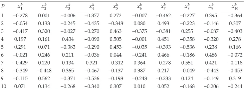
Now we useAlgorithm 3.4on the same variational inequalities except that
Fx:τxDx−Mxq, 4.8
Table 1:Numerical results:Algorithm 3.4withn10.
P xk
1 x k
2 xk3 xk4 x k
5 xk6 xk7 x8k xk9 xk10 1 −0.278 0.001 −0.006 −0.377 0.272 −0.007 −0.462 −0.227 0.395 −0.364 2 −0.054 0.133 −0.245 −0.435 −0.348 0.080 0.493 −0.223 −0.146 0.307 3 −0.417 0.320 −0.027 −0.270 0.463 −0.375 −0.381 0.255 −0.087 −0.403 4 0.197 0.161 0.434 −0.090 0.505 −0.001 0.451 −0.358 −0.320 0.278 5 0.291 0.071 −0.383 −0.290 0.453 −0.035 −0.393 −0.536 0.238 0.166 6 −0.021 0.246 0.211 −0.036 0.044 −0.241 0.466 −0.186 0.486 −0.072 7 −0.429 0.220 0.134 0.321 −0.312 0.364 −0.278 0.551 0.421 −0.118 8 −0.349 −0.448 0.365 −0.467 −0.137 0.387 0.217 −0.049 −0.443 −0.453 9 −0.115 0.562 −0.371 −0.536 −0.198 −0.248 −0.233 0.124 −0.149 0.319 10 0.071 0.134 −0.268 −0.340 0.307 0.010 0.052 −0.168 −0.206 −0.244
Withx 0,0,0,0,0,0,0,0,0,0 ∈ intCand the tolerance 10−6, we obtained the computational resultssee, theTable 1.
Acknowledgments
The authors would like to thank the referees for their useful comments, remarks and suggestions. This work was completed while the first author was staying at Kyungnam University for the NRF Postdoctoral Fellowship for Foreign Researchers. And the second author was supported by Kyungnam University Research Fund, 2010.
References
1 P. N. Anh, L. D. Muu, and J.-J. Strodiot, “Generalized projection method for non-Lipschitz multivalued monotone variational inequalities,”Acta Mathematica Vietnamica, vol. 34, no. 1, pp. 67–79, 2009.
2 P. N. Anh, L. D. Muu, V. H. Nguyen, and J. J. Strodiot, “Using the Banach contraction principle to implement the proximal point method for multivalued monotone variational inequalities,”Journal of Optimization Theory and Applications, vol. 124, no. 2, pp. 285–306, 2005.
3 J. Y. Bello Cruz and A. N. Iusem, “Convergence of direct methods for paramontone variational inequalities,”Computational Optimization and Applications, vol. 46, no. 2, pp. 247–263, 2010.
4 F. Facchinei and J. S. Pang,Finite-Dimensional Variational Inequalities and Complementary Problems, Springer, New York, NY, USA, 2003.
5 M. Fukushima, “Equivalent differentiable optimization problems and descent methods for asymmet-ric variational inequality problems,”Mathematical Programming, vol. 53, no. 1, pp. 99–110, 1992.
6 I. V. Konnov,Combined Relaxation Methods for Variational Inequalities, Springer, Berlin, Germany, 2000.
7 J. Mashreghi and M. Nasri, “Forcing strong convergence of Korpelevich’s method in Banach spaces with its applications in game theory,”Nonlinear Analysis: Theory, Methods & Applications, vol. 72, no. 3-4, pp. 2086–2099, 2010.
8 M. A. Noor, “Iterative schemes for quasimonotone mixed variational inequalities,”Optimization, vol. 50, no. 1-2, pp. 29–44, 2001.
9 D. L. Zhu and P. Marcotte, “Co-coercivity and its role in the convergence of iterative schemes for solving variational inequalities,”SIAM Journal on Optimization, vol. 6, no. 3, pp. 714–726, 1996.
10 P. Daniele, F. Giannessi, and A. Maugeri, Equilibrium Problems and Variational Models, vol. 68 of
Nonconvex Optimization and Its Applications, Kluwer Academic Publishers, Norwell, Mass, USA, 2003.
12 C. J. Goh and X. Q. Yang,Duality in Optimization and Variational Inequalities, vol. 2 of Optimization Theory and Applications, Taylor & Francis, London, UK, 2002.
13 A. N. Iusem and M. Nasri, “Inexact proximal point methods for equilibrium problems in Banach spaces,”Numerical Functional Analysis and Optimization, vol. 28, no. 11-12, pp. 1279–1308, 2007.
14 J. K. Kim and K. S. Kim, “New systems of generalized mixed variational inequalities with nonlinear mappings in Hilbert spaces,”Journal of Computational Analysis and Applications, vol. 12, no. 3, pp. 601– 612, 2010.
15 J. K. Kim and K. S. Kim, “A new system of generalized nonlinear mixed quasivariational inequalities and iterative algorithms in Hilbert spaces,”Journal of the Korean Mathematical Society, vol. 44, no. 4, pp. 823–834, 2007.
16 R. A. Waltz, J. L. Morales, J. Nocedal, and D. Orban, “An interior algorithm for nonlinear optimization that combines line search and trust region steps,”Mathematical Programming, vol. 107, no. 3, pp. 391– 408, 2006.
17 P. N. Anh, “An interior proximal method for solving monotone generalized variational inequalities,”
East-West Journal of Mathematics, vol. 10, no. 1, pp. 81–100, 2008.
18 A. Auslender and M. Teboulle, “Interior projection-like methods for monotone variational inequali-ties,”Mathematical Programming, vol. 104, no. 1, pp. 39–68, 2005.
19 A. Bnouhachem, “An LQP method for pseudomonotone variational inequalities,”Journal of Global Optimization, vol. 36, no. 3, pp. 351–363, 2006.
20 A. N. Iusem and M. Nasri, “Augmented Lagrangian methods for variational inequality problems,”
RAIRO Operations Research, vol. 44, no. 1, pp. 5–25, 2010.
21 J. K. Kim, S. Y. Cho, and X. Qin, “Hybrid projection algorithms for generalized equilibrium problems and strictly pseudocontractive mappings,”Journal of Inequalities and Applications, vol. 2010, Article ID 312062, 17 pages, 2010.
22 J. K. Kim and N. Buong, “Regularization inertial proximal point algorithm for monotone hemicontinuous mapping and inverse strongly monotone mappings in Hilbert spaces,”Journal of Inequalities and Applications, vol. 2010, Article ID 451916, 10 pages, 2010.
23 Y. Nesterov, “Dual extrapolation and its applications to solving variational inequalities and related problems,”Mathematical Programming, vol. 109, no. 2-3, pp. 319–344, 2007.
24 J.-P. Aubin and I. Ekeland,Applied Nonlinear Analysis, Pure and Applied Mathematics, John Wiley & Sons, New York, NY, USA, 1984.
25 P. N. Anh and L. D. Muu, “Coupling the Banach contraction mapping principle and the proximal point algorithm for solving monotone variational inequalities,”Acta Mathematica Vietnamica, vol. 29, no. 2, pp. 119–133, 2004.
26 G. Cohen, “Auxiliary problem principle extended to variational inequalities,”Journal of Optimization Theory and Applications, vol. 59, no. 2, pp. 325–333, 1988.
27 O. L. Mangasarian and M. V. Solodov, “A linearly convergent derivative-free descent method for strongly monotone complementarity problems,”Computational Optimization and Applications, vol. 14, no. 1, pp. 5–16, 1999.