A class of derivative free trust region methods with interior backtracking technique for nonlinear optimization problems subject to linear inequality constraints

R E S E A R C H

Open Access

A class of derivative-free trust-region

methods with interior backtracking

technique for nonlinear optimization

problems subject to linear inequality

constraints

Jing Gao

_{and Jian Cao}

*_{Correspondence:}

[email protected]

2_{School of Information Technology}

and Media, Beihua University, Jilin, P.R. China

Full list of author information is available at the end of the article

Abstract

This paper focuses on a class of nonlinear optimization subject to linear inequality constraints with unavailable-derivative objective functions. We propose a derivative-free trust-region methods with interior backtracking technique for this optimization. The proposed algorithm has four properties. Firstly, the derivative-free strategy is applied to reduce the algorithm’s requirement for first- or second-order derivatives information. Secondly, an interior backtracking technique ensures not only to reduce the number of iterations for solving trust-region subproblem but also the global convergence to standard stationary points. Thirdly, the local convergence rate is analyzed under some reasonable assumptions. Finally, numerical experiments demonstrate that the new algorithm is effective.

MSC: 49M37; 65K05; 90C30; 90C51

Keywords: Affine scaling; Trust-region method; Inequality constraints; Derivative-free optimization; Interior backtracking technique

1 Introduction

In this paper, we analyze the solution of following nonlinear optimization problem:

min f(x)

s.t. Ax≥b,

(1)

wheref(x) is a nonlinear twice continuously differentiable function, but its first-order or second-order derivatives are not explicitly available,Adef= [aT

1,aT2, . . . ,aTm]T∈ m×nwith aT

i ∈ nandb def

= [b1,b2, . . . ,bm]T∈ m. The feasible set, in (1), is denoted bydef= {x∈ n_{|Ax≥b}and the strict interior feasible set isint()}def_={x∈ n_|Ax>b}.

1.1 Affine-scaling matrix for inequality constraints The KKT system of (1) is

∇f(x) –ATλf= 0,

diag{Ax–b}λf= 0, (2)

Ax–b≥0, λf≥0,

whereλf ∈ m. A feasibilityx∗is said to be the stationary point for problem (1), if there

exists a vector 0≤λf∗∈ msuch that the KKT system (2) holds.

To solve this KKT system, some effective affine-scaling algorithms are designed. Ref-erence [1] proposed an affine-scaling trust-region method with interior-point technique for bound-constrained semismooth equations. Reference [2] introduced affine-scaling interior-point Newton methods for bound-constrained nonlinear optimization. In par-ticular, [3] proved the superlinear and quadratic convergence properties of affine-scaling interior-point Newton methods for bound optimization problems without strict comple-mentarity assumption. Different affine-scaling matrix denotes different algorithm. In [4], the Dikin affine scaling was denoted by

D(x)def= diag{Ax–b} and Dkdef=D(xk). (3)

Moreover, diagonal matrixCfk def

= diag{|λfk|}was presented in [4]. Thenλfk could be

ob-tained as a least-squares Lagrangian multiplier approximation computed by

AT

–D

1 2

k

λfk

L.S.

=

∇fk

0

. (4)

One efficient affine-scaling interior-point trust-region model is the one which is presented in [5] and [6], written in the form

min qfk(p) =∇f T k p+

1 2p

T_H fkp+

1 2p

T_AT_D–1 k CfkAp

subject to p;D–

1 2

k Ap≤k,

(5)

where∇f(xk) is the gradient off(x) at the current iteration,Hfk is either∇2f(xk) or its

approximation. Furthermore,∇fT

k hfk ≤ε, where

hfk= –

∇f(xk) –ATλfk

, (6)

andεis a small enough constant, is usually considered as the termination criterion in this class of algorithms.

(1). If both the feasibility and the stability of the algorithm need to be guaranteed, we should consider the derivative-free trust-region methods.

1.2 Derivative-free technique for trust-region subproblem

Since the first- or second-order derivatives of objective functions are not explicitly avail-able, the derivative-free optimization algorithms have been favored by researchers for a time. The application forms of the derivative-free theory are devise [7, 8] and widely ap-plied. Reference [9] proposed a derivative-free algorithm for least-squares minimization, and proved the local convergence in [10]. Reference [11] presented a derivative-free ap-proach to constrained multiobjective nonsmooth optimization. Reference [12] presented a higher-order contingent derivative of perturbation maps in multiobjective optimization. In [13], Conn proposed an unconstrained derivative-free trust-region method. They con-structed the trust-region subproblem

min

s∈B(0;k)

mk=m(xk+s) =m(xk) +sTgk+

1 2s

T_H mks

by using a polynomial interpolation technique, where∇m(xk) =gk, and∇2m(xk) =Hmk.

Following this idea, we consider thatYk={y0k,y1k, . . . ,ytk}is an interpolation sample set

around the current iteration pointxk, and we construct the trust-region subproblem

min qmk(p) =g T kp+

1 2p

T_H mkp+

1 2p

T_AT_D–1 k CmkAp

s.t. p;D–

1 2

k Ap≤k.

(7)

Cmk def

= diag{|λmk|}withλmkobtained from

AT

–D

1 2

k

λmk

L.S.

=

gk

0

, (8)

hmk = –

gk–ATλmk

. (9)

We should note that the gradient and Hessian in (5) and (7), (4) and (8), (6) and (9) are different. Meanwhile, since the algorithm in this paper adopts both the decrease direction

pand the stepsizeα to update the iteration point, we give a new definition of the error

bounds between the objective functionf(xk+αp) and the approximation functionm(xk+

αp) to ensure the global convergence. We shall show the details after assumption (A1).

Assumption

(A1) Suppose that a level setL(x0)and a maximal radiusmaxare given. Assume thatf is twice continuously differentiable with Lipschitz continuous Hessian in an appropriate open domain containing themaxneighborhood _x∈L(x0)B(x,max) of the setL(x0).

Definition 1 Given a functionfsatisfies (A1).M={m:n_{→ ,m∈C}2_{}is a set of model}

functions. If there exist positive constantsκef,κeg,κeh, andκblh, such that, for anyx∈L(x0),

∈(0,max], andα∈(0, 1], there is a model functionm(x+αp)∈M, with Lipschitz

1 the error between the Hessian of the modelm(x+αp)and the Hessian of the function f(x+αp)satisfies

_∇2_{f(x+αp) –∇}2_{m(x+αp)≤κ}

ehα, ∀p∈B(0,); (10)

2 the error between the gradient of the modelm(x+αp)and the gradient of the functionf(x+αp)satisfies

_∇f(x+αp) –∇m(x+αp)≤κegα22, ∀p∈B(0,); (11)

3 the error between the modelm(x+αp)and the functionf(x+αp)satisfies

f(x+αp) –m(x+αp)≤κefα33, ∀p∈B(0,). (12)

Such a modelmis called fully quadratic onB(x,).

In this paper, we aim to present a class of derivative-free trust-region method for nonlin-ear programming with linnonlin-ear inequality constraints. The main features of this paper are:

• We use the derivatives of approximation functionm(xk+αp)to replace the

derivatives of objective functionf(xk+αp)to reduce the algorithm’s requirement for gradient and Hessian of the iteration points. We solve an affine-scaling trust-region subproblem to find a feasible search direction in each iteration.

• In thekth iteration, a feasible search directionpis obtained from an affine-scaling trust-region subproblem. Meanwhile, interior backtracking skill will be applied both for determining stepsizeαand for guaranteeing the feasibility of iteration point. • We will show that the iteration points generated by the proposed algorithm could

converge to the optimal points of (1).

• Local convergence will be given under some reasonable assumptions.

This paper is organized as follows: we describe a class of derivative-free trust-region method in Sect. 2. The main results including global convergence property and local con-vergence rate will be discussed in Sect. 3. The numerical results will be illustrated in Sect. 4. Finally, we give some conclusions.

Notation In this paper, · is the 2-norm for a vector and the induced 2-norm for a matrix. B⊂ n_{is a closed ball andB(x,) is the closed ball centered atx, with radius}

> 0.Yis a sample set andL(x0) ={x∈ n_{|f(x)≤f(x0),Ax≥b}is the level set about the}

objective functionf. We use the subscriptfkand subscriptmkto distinguish the relevant

information between the original function and the approximate function. For example,

Hfk is the Hessian off atkth iteration andHmk is the Hessian ofmkatkth iteration.

2 A derivative-free trust region method with interior backtracking technique To solve the optimization problem (1) with not all available first- or second-order deriva-tives, we design a derivative-free trust-region method. An affine-scaling matrix is denoted by (3) for linear inequality constraints. We chose a stepsizeαksatisfying the following

in-equalities:

f(xk+αkpk)≤f(xk) +αkκ1gkTpk, (13a)

Moreover, set

θk=

⎧ ⎨ ⎩

1, ifxk+αkpk∈int(),

1 –O(pk2), otherwise,

(14)

whereθk∈(θ0, 1], for some 0 <θ0< 1. Theθkis to ensure the iterative points generated

by the algorithm are strictly interior. Combining with (13a), (13b) and (14), this interior backtracking technique is to guarantee the feasibility of the iterative points. The algo-rithm possesses the trust-region property and the derivative-free technique is reflected

in the trust-region subproblem (7) since the gradientgkand HessianHmk come from the

approximation function, which are different from∇fkandHfk in (5), satisfying the error

bounds (11) and (12). We adoptg_kThmkto be a termination criterion. Now we present

the derivative-free trust-region method in detail (see Algorithm 1).

Remark1 We add a backtracking interior line-search technique in the algorithm. It is helpful to reducing the number of iterations. Equation (13a) is used to guarantee the de-scent property off(x) and (13b) ensures the feasibility ofxk+αkpk.

Remark2 The scalarαk, given in step 5, denotes the stepsize alongpk to the boundary

(13b) of the linear inequality constraints

kdef= min

–a

T ixk–bi

aT ipk

–a

T ixk–bi

aT i pk

> 0,i= 1, 2, . . . ,m

, (15)

with kdef= +∞if –(aTi xk–bi)/(aTi pk)≤0 for alli= 1, 2, . . . ,m. A key property of the scalar

αkis that an arbitrary stepαkpkto the pointxk+αkpkdoes not violate any linear inequality

constraints.

Remark3 Let

Mmk=

Hmk 0

0 Cmk

. (16)

The first-order necessary conditions of (7) implies that there existsvmk≥0 such that

(Mmk+vmkI)

pk ˆ pk

= –

gk

0

+

AT

–D

1 2

k

λmk+1, with

vmk

k–

pk ˆ pk

= 0.

(17)

In order to obtain a suitable approximation function, Algorithm 1 needs to update the objective function of the trust-region subproblem if necessary. The model-improvement algorithm is applied only ifgT

khmk ≤εand at least one of the following holds: The model m(xk+αp) is not certifiably fully quadratic onB(xk,k) ork>ιgkThmk. It improves on

the current approximate functionm(xk+αp) to meet the requirements of the error bounds

Algorithm 1Derivative-free trust-region method with interior backtracking technique

1 Initialization:Givenx0,max> 0,0∈(0,max],0≤η0≤η1< 1, (η1= 0) and

θ0∈(0, 1)are constants.k:= 0.

2 Construct model function:Letyk=xk, and obtain an interpolation point set Yk={y0_k, . . . ,yt_k}. Construct a quadratic functionm(xk+αp), get the information such asgk,Hmk. CalculateDk,λmkandhmk from (3), (8) and (9).

3 Termination criterion:Ifg_kThmk>ε, then go to step 4. Consider the modelmkon B(xk,k), there are two cases would be happened:

(a) Ifmkis not fully quadratic onB(xk,k)ork>ιgkThmkholds, construct another model to modifiedmk,k=min{max{ ˜k,β˜g_kThm˜k},k}and go to step 4.

(b) Otherwise, we get the optimal point and stop.

4 Trust-region subproblem:solve trust-region subproblem (7) to find descent direction pk.

5 Step size:chooseαk= 1,α,α2, . . ., until the inequalities (13a) and (13b) are satisfied. 6 Setsk=αkθkpkby (14).

7 CalculatePred(sk) =m(xk) –m(xk+sk),Ared(sk) =f(xk) –f(xk+sk),

ρk=

Ared(sk)

Pred(sk)

.

(a) Ifρk≥η1or if bothρk≥η0andmkis fully quadratic onB(xk,k), then set yk+1=xk+1=xk+sk, go to step 2.

(b) Otherwisexk+1=xk.

8 Ifρk<η1, call Algorithm 2 to guaranteemkis fully quadratic. (a) Ifmkis not fully quadratic, modifyk.

(b) Otherwise, setmk+1=mk. 9 Trust-region radius update:set

k+1∈

⎧ ⎪ ⎪ ⎪ ⎪ ⎪ ⎨ ⎪ ⎪ ⎪ ⎪ ⎪ ⎩

min{ς k,max} ifρk≥η1andk<ιgkThmk,

[k,min{ς k,max}] ifρk≥η1andk≥ιgkThmk,

ζ k ifρk<η1andmkis fully quadratic,

k ifρk<η1andmkis not fully quadratic.

10 Setk:=k+ 1and go to step 2.

Algorithm 2Model-improvement mechanism

1 Initialization: seti= 0,m(0)_k =mk.

2 Repeat:i=i+ 1;k=ωi–1k; Ensurem(ki–1)satisfies the error bounds (10)–(12) in Definition 1 onB(xk,ωi–1k).

Untilk≤ι(gkThmk) (i)_.

3 Main results and discussion

In this section, we mainly discuss some properties about the proposed algorithm, includ-ing the discussion of the error bounds, the sufficiently descent property, the global and local convergence properties. First of all, we make some necessary assumptions as follows.

Assumptions

(A2) The level setL(x0)is bounded.

(A3) There exist positive constantsκgf andκgmsuch that∇fk ≤κgf andgk ≤κgm, respectively, for allxk∈L(x0).

(A4) There exist positive constantsκHf andκHg such thatHfk ≤κHf and Hmk ≤κHm, respectively, for allxk∈L(x0).

(A5) [_A–D12

k]is full row rank for allxk∈L(x0).

3.1 Error bounds

Observe first that some error bounds hold immediately.

Lemma 1 Suppose that(A1)–(A5),the error bounds(10)–(12)and the fact thatk≤max hold.If mkis a fully quadratic model on B(xk,k),then the following bound is true:

hfk–hmk ≤κhαkk. (18)

Proof Using the theory of matrix perturbation analysis, Eqs. (4) and (8), we obtain

λfk–λmk ≤AA T_+D

k

–1

A∇f(xk) –gk, (19)

whereAAT is a positive definition matrix andDkis a diagonal matrix related withxk∈

L(x0). By (A2), there exists a constantκλ> 0 such that(AAT+Dk)–1A ≤κλ. Thus,

from (6), (9) and the error bound (11), one has the fact that

hfk–hmk=∇f(xk) –gk–A T_(λ

fk–λmk)

≤∇f(xk) –gk+κλA∇f(xk) –gk ≤1 +κλA∇f(xk) –gk

≤1 +κλA

κegα2k2k

≤1 +κλA

κegmaxαkk.

Clearly, the conclusion holds withκh= (1 +κλA)κegmax.

Lemma 2 Suppose that(A1)–(A5),the error bounds(10)–(12)and the fact thatk≤max hold.If mkis a fully quadratic model on B(xk,k),for some constantκ2,one has

_∇f(xk)Thfk–g T

khmk≤κ2αkk. (20)

Proof Using the triangle inequality, Cauchy–Schwarz inequality, (18), (A3), the error bounds (10)–(12) and the fact thatαk∈(0, 1] andk≤maxsuccessively, we obtain

≤∇f(xk) –gkhfk+gkhmk–hfk ≤∇f(xk) –gkhfk+κhαkkgk ≤(κegκgfmax+κgmκh)αkk,

which implies that the inequality (20) holds withκ2=κegκgfmax+κgmκh.

Lemma 3 Suppose that(A1)–(A5),the error bounds(10)–(12)and the fact thatk≤max hold.If∇f_kThfk = 0,then step3of Algorithm1will stop in a finite number of improvement steps.

Proof Now we should prove that∇fT

k hfkmust be zero if the loop of Algorithm 2 is

infinite.

In fact, there are two cases could cause Algorithm 2 to be implemented. One is that

mk is not fully quadratic, the other is that the radius k>ιgTkhmk. Then set m (0) k = mk, and improve the model to be fully quadratic onB(xk,k), which denoted bym(1)k .

If (g_kThmk)(1) ofm (1)

k satisfies the inequalityι(gTkhmk)(1) ≥k, Algorithm 2 stops with

k=k≤ι(g_kThmk) (1)_.

Otherwise,ι(gT khmk)

(1)_<

kholds. Algorithm 2 will improve the model onB(xk,ωk)

and the resulting model is denoted bym(2)_k . Ifm(2)_k satisfiesι(g_kThmk)

(2) _≥ω

k, the

pro-cedure stops. If not, the radius should be multiplied byωand Algorithm 2 will improve

the model onB(xk,ω2k), and go on.

The only case for Algorithm 2 to be infinite is if

ιg_kThmk

(i)

<ωi–1k for alli≥1.

It implies

lim

i→+∞

g_kThmk

(i)

= 0.

By the bound (20)∇fT

k hfk– (g T khmk)

(i) _≤κ

2ωi–1αkk for alli≥1, we obtain

_∇f_kThfk≤∇f T k hfk–

g_kThmk

(i)

+gT_khmk

(i)

≤κ2ωi–1αkk+

ωi–1

ι k

≤κ2ωi–1k+

ωi–1

ι k

≤

κ2+

1 ι

ωi–1k.

By the choice ofω∈(0, 1) the above inequality means that∇f_kThfk= 0. The conclusion

shows us step 3 will stop in a finite number of improvements.

3.2 Sufficiently descent property

obtained in [6] if steppkis the optimal point of the trust-region subproblem (7), there is a

constantκ3> 0 such that

g_kTpk≤–κ3gkThmk

1 2_min

k,

g_kThmk

1 2

Mmk

. (21)

Lemma 4 Suppose that(A1)–(A5)and the error bounds(10)–(12)hold.pkis the solution of the trust-region subproblem(7).Then there must exist an appropriateαk> 0which satisfied inequalities(13a).

Proof We start by considering the maximal step-length along the trust-region subproblem descent direction that preserves sufficient feasibility in the sense of the (13a). Successively using the mean value theorem and (11), we obviously obtain

f(xk) –f(xk+αpk)

= –α∇f(xk)Tpk–

1 2α

2_pT

k∇2f(ξk)pk

≥–κegα33k–αgkTpk–

1 2α

2_pT

k∇2f(ξk)pk

= –ακ1gT_kpk–κegα33k+α(κ1– 1)gkTpk–

1 2α

2_pT

k∇2f(ξk)pk, (22)

whereξk∈(xk,xk+sk).

There are two cases that may be considered. The first ispT_k∇2f(ξk)pk≤0. By canceling

the last term of Eqs. (22), (21), g

T khmk

1 2

κλmκHm ≤kfor large enoughkand the fact thatk≤

max, it is thus easy to see that there exists anα∗= [

κ3(1–κ1)κHmκλm κegmax ]

1

2 _{> 0 such that (13a)}

holds. The second case ispT

k∇2f(ξk)pk> 0. Using the Cauchy–Schwarz inequality and the

fact thatαk∈(0, 1] andk≤max, we deduce that

f(xk) –f(xk+αpk) +ακ1gkTpk

≥–κegα33k+α(κ1– 1)gkTpk–

1 2α

2_κ Hfpk

2

≥–κegα2max2_k+α(κ1– 1)gkTpk–

1 2α

2_κ Hf

2 k

=α

–κegmax–

1 2κHf

2_kα+ (κ1– 1)gkTpk

≥0,

whenα∗=κ3(1–κ1)κHmκλm

κegmax+12κHf > 0. Thus the final conclusion obtained.

We therefore see that it is reasonable to design line-search step criterion in step 5, which provided us a nonincreasing sequence{f(xk)}.

Lemma 5 Let step pkbe the solution of the trust-region subproblem(7).Suppose that(A1)–

sufficiently descent condition:

Pred(sk)≥κ4αkθkgkThmk

1 2_min

k,

g_kThmk

1 2

Mmk

, (23)

for all gk,hmk,Mmk,andk.

Proof Combining now (7), (17), Lemma 4,θk∈(θ0, 1] and the fact thatαk≤1, we get

Pred(sk) = mk–m(xk+sk)

= –αkθkgkTpk–

(αkθk)2

2 p

T kMmkpk

(17)

= –αkθkgkTpk+

(αkθk)2

2 g

T kpk+

(αkθk)2

2 vmk

pk ˆ pk 2

≥ αkθk

αkθk

2 – 1

g_kTpk

≥ 1

2κ3αkθkg

T khmk

1 2_min

k,

gT khmk

1 2

Mmk

= κ4αkθkgkThmk

1 2_min

k,

gT khmk

1 2

Mmk

.

3.3 Global convergence

Every iteration point in thek+ 1th iteration will be chosen on the regionB(xk,αkk).

Following the lemma one first shows that the current iteration must be successful ifαkk

is small enough.

Lemma 6 Suppose that (A1)–(A5) and the error bounds (10)–(12) hold. mk is fully quadratic on B(xk,k),gkThmk = 0and

αkk≤k≤min

1 κHmκλm

,κ4(1 –η1) 2κef2max

g_kThmk

1 2_,

whereκλm is the bound of Cmk,for all x∈L(x0).Then the kth iteration is successful.

Proof We notice that, for allk and the model functionmk, one hasf(xk) =m(xk). Let Mfk=

H_fk 0 0 C_fk

, from (16) and (A3), we know thatMmk ≤κHmκλm. Thus combiningk≤

gT_kh_mk12

κ_Hmκλm with the sufficient decrease condition (23), we immediately get

Pred(sk)≥κ4αkθkgkThmk

1 2_min

k,

g_kThmk

1 2

Mmk

≥κ4αkθkgkThmk

1 2

k.

Using Eqs. (12), (23), the fact thatαk∈(0, 1] andθk∈(0, 1], we have

|ρk– 1| =

f(xk) –f(xk+1) m(xk) –m(xk+1)

≤ f(xk) –m(xk) m(xk) –m(xk+1)

+m(xk+1) –f(xk+1)

m(xk) –m(xk+1)

f(xk)=m(xk)

≤ 2κefαk3θk33k

κ4αkθkgkThmk

1 2_k

θk≤1

≤ 2κef2maxαkk

κ4gkThmk

1 2

≤ 1 –η1.

Thusρk≥η1and the iteration is successful.

Lemma 7 Suppose that(A1)–(A5)and the error bounds(10)–(12)hold.If the number of successful iteration is finite,then

lim

k→+∞∇f(xk)

T_h fk= 0.

Proof We consider that all the model-improving iterations before mk becomes fully

quadratic are less than a constant N. Suppose that the current iteration is an iteration

after a successful one. It means that an infinite number of iterations are acceptable or not nice. In these two cases,kis shrinking. Furthermore,kis reduced by a factorζat least

once everyNiterations, which impliesk→0.

For thejth iteration, we denote theith iteration afterjby the indexij, then

xj–xij ≤Nj→0, j→+∞.

Using the triangle inequality, we obtain

_∇f(xj)Thfj≤∇f(xj) T_h

fj–∇f(xj) T_h

f_ij+∇f(xj)Thf_ij+∇f(xij) T_h

f_ij

+∇f(xij) T_h

f_ij–giTjhfij+g T ijhfij–g

T

ijhmij+g T ijhmij.

The following work is to show that all these terms on the right-hand side are converging to zero. Because of the Lipschitz continuity of∇f and the fact thatxij–xj →0 the first and

second terms converge to zero. The inequalities (10) and (11) imply the third and fourth terms on the right-hand side are converging to zero. According to Lemma 3, ifgT

ijhmij

0 for small enoughij,ijwould be a successful iteration, which yield a contradiction. Thus

the last term converges to zero.

Lemma 8 Suppose that(A1)–(A5),the error bounds(10)–(12)and(23)hold.Suppose fur-thermore that the strict complementarity of the problem(1)holds.Then

lim inf

k→+∞g

T

khmk= 0.

Proof The key is that we may find a contradiction with the fact that{f(xk)}is a

nonincreas-ing bounded sequence unlessxkis a stationary point. We thus have to verify that there

We observe from (13a), Lemma 4 and (21) that

f(xk) –f(xk+αkpk)≥–αkκ1gkTpk

≥αkκ1κ3gTkhmk

1 2_min

k,

gT khmk

1 2

Mmk

≥αkκ1κ3min

k,

Mmk

→0. (24)

Thus from (24), two cases should be considered next, that is,

lim inf

k→∞ αk= 0 (25)

and

lim

k→∞k= 0. (26)

We now start the proof of (25). On one hand,αkis accepted by (13b) the boundary of

inequality constraints alongpk. From Eq. (15)

k=min

–a

T ixk–bi

aT_ipk

–a

T i xk–bi

aT_ipk

> 0,i= 1, 2, . . . ,m

,

withαk= +∞if –(aTixk–bi)/(aTipk)≤0 for alli= 1, 2, . . . ,m,pˆk=D –12

k Apk and (17), we

know that there existsλmk+1such that

aT_ipk=

aT_i pk–bi

1 2_pˆi

k= –

(aT

ipk–bi)λimk+1

vmk+|λimk+1| ,

wherepˆi_kandλi

mk+1are theith components of the vectorspˆkandλmk+1, respectively. Hence, there existsj∈1, . . . ,msuch that

αk= –

aT_jxk–bj aT

jpk ≥

vmk+|λ j mk+1|

λjmk+1

≥vmk+|λ j mk+1|

λmk+1∞

. (27)

From (17), we have

AT

–D

1 2

k

λmk+1= –

gk

0

+ (Mmk+vmkI)

pk ˆ pk

.

Since [_A–D12

k]

T_{is full row rank for allx∈L(x0),λ}

mk is bounded andm(x) is twice

contin-uously differentiable, there existκ5> 0 andκ6> 0 such that

Using the fact thatvmk(k–

pk

ˆ

pk

) = 0 and taking the norm to both sides of (17), we

deduce that

vmkk =vmk

pk ˆ pk

≥gk–ATλmk 2

+D

1 2

kλmk

212 _–M

mk(pk;pˆk)

=g_kThmk

1 2 _–M

mk(pk;pˆk).

And noting(pk;pˆk) ≤k, we can obtain

vmk≥ gT

khmk

1 2

k

–Mmk.

Combining the assumptiongT

khmk>

2_with

k→0 deduced from (24), it is clear from

the factMmk ≤κλmκHmthat, for∀k,

lim

k→∞vmk= +∞.

Thus (27) implies that

lim

k→∞αk= 0.

Furthermore,k→0 means thatlimk→∞pk= 0, from which we deduce that, for some

0 <θ0< 1 andθk– 1 =O(pk2), the strictly feasible stepsizeθk∈(θ0, 1]→1. From the

above, we have already seen that (25) holds in the case thatαkis determined by (13b).

There is another case thatαk is determined by (13a). In this case, we are able to verify

thatαk= 1 is acceptable whenksufficiently large. If not,

κ1g_kTpk<f(xk+pk) –f(xk)

must hold. Applying the Taylor series, (10)–(11), (A3) and the fact thatk≤max, we

deduce that

κ1g_kTpk < f(xk+pk) –f(xk) =∇f(xk)Tpk+

1 2p

T

k∇2f(ξk)pk

≤

κegmax+

1

2κehmax+ 1 2κHm

2_k+g_kTpk,

whereξk∈(xk,xk+sk). This inequality is equivalent to the form of

(1 –κ1)gkTpk+

κegmax+

1

2κehmax+ 1 2κHm

2_k> 0.

Moreover, (21) andg_kThmk ≥

2_{imply that}

–(1 –κ1)κ3min

k,

κHm

+

κegmax+

1

2κehmax+ 1 2κHm

Thus ifk≤_2κegmax2(1–κ+κeh1)κ3max +κHm ≤

κ_Hm we deduce from the inequality

k

k

κegmax+

1

2κehmax+ 1 2κHm

– (1 –κ1)κ3

> 0

that

k>

2(1 –κ1)κ3

2κegmax+κehmax+κHm

.

Clearly, a contradiction appears here. It implies thatαk= 1 forksufficiently large.

There-fore (25) always holds.

On the other hand, we should prove that (26) is true. From step 3 of Algorithm 1, we know that

k≥ιgkThmk.

By the assumption thatgT

khmk ≥

2_{, we obtain}

k≥ι.

Wheneverkfalls below a constantκ¯7given by

¯

κ7=min

κHmκλm

,κ4(1 –η1) 2κef2max

,

thekth iteration is either successful or model-improving, and hence from step 9, we are

able to deduce both thatk+1≥kandk+1≥ζ k. Combining with the rules of step 9

we conclude thatk+1≥min{ι,ζκ¯7}=κ7. It means thatk0, ifgkThmk ≥ 2_.

In conclusion, the sequence{f(xk)}is not convergent if we suppose thatgkThmk ≥ 2_,

which contradicts the fact that{f(xk)}is a nonincreasing bounded sequence. It implies

that

lim inf

k→+∞

g_kThmk= 0.

Lemma 9 For any subsequence{ki}such that

lim

i→+∞g

T

kihmki= 0, (28)

we also have

lim

i→+∞

_∇f_kT_ihf_ki= 0. (29)

Proof First, we note that, by (28),g_kT_ihm_ki ≤εwhenisufficiently large. Thus the

criti-cality step ensures that the modelmkiis a fully quadratic function on the ballB(xki,ki),

withki≤ιg T

kihmkifor allisufficiently large (if∇f T

kihfki = 0). Then, using the bound

(20) on the error between the terminal conditions of function and model, we have

_∇f_kT_ihf_ki–gkTihmki≤κ2αkiki≤κ2ιαkig T

As a consequence, we have _∇f_kT_ihf_ki=∇fkTihfki–g

T

kihmki+g T

kihmki≤(κ2αkiι+ 1)g T kihmki

≤(κ2ι+ 1)gkTihmki

for allisufficiently large. ButgT

kihmki →0 implies (29) holds.

Then we obtain the global convergence derived from Lemmas 8 and 9.

Theorem 1 Suppose that(A1)–(A5),the error bounds(10)–(12)and(23)hold.Suppose furthermore that the strict complementarity of the problem(1)holds. Let{xk} ⊂ n be sequence generated by Algorithm1.Then

lim inf

k→+∞∇f

T k hfk= 0.

The above theorem shows us there exists a limit point that is first-order critical. In fact, we are able to prove that all limit points of the sequence of iterations are first-order critical.

Theorem 2 Suppose that(A1)–(A5),the error bounds(10)–(12)and(23)hold.Suppose furthermore that the strict complementarity of the problem(1)holds. Let{xk} ⊂ n _be sequence generated by Algorithm1.Then

lim

k→+∞∇f

T

k hfk= 0.

Proof We first obtained from Lemma 7 that the theorem holds in the case whenSis finite.

Hence, we will assume thatSis infinite. For the purpose of deriving a contradiction, we

suppose that there exists a subsequence{ki} of successful or acceptable iterations such that

_∇f_kT_ihf_ki≥12> 0 (30)

for some1> 0 and for alli. Then, because of Lemma 9, we obtain

g_kT_ihm_ki≥22> 0

for some2> 0 and for allisufficiently large. Without loss of generality, we pick2such

that

2₂≤min

₁2 2(2 +κegι)

,

. (31)

Lemma 8 then ensures the existence, for each{ki}in the subsequence, of a first iteration i>kisuch thatgTihm_i<

2

2. By removing elements from{ki}, without loss of

general-ity and without a change of notation, we thus see that there exists another subsequence indexed by{i}such that

g_kThmk≥ 2

2 forki≤k≤iandgTihm_i<

2

2, (32)

We now restrict our attention to the setKcorresponding to the subsequence of itera-tions whose indices are in the set

i∈N0

{k∈N0:ki≤k≤i},

wherekiandibelong to the two subsequences given above in (31).

We know that g_kThmk ≥ 2

2 for k∈K. From Lemma 8 limk→+∞αkk = 0 and by

Lemma 5 we conclude that for any large enoughk∈Kthe iterationkis either successful if

the model is fully quadratic or model-improving otherwise. Moreover, for eachk∈K∩S

we have

f(xk) –f(xk+sk)≥η1

m(xk) –m(xk+hk)

≥η1κ4αkθkgTkhmk

1 2_min

k,

gT khmk

1 2

Mmk

,

and, for any suchklarge enough,k≤κ_hmκ2λm. Hence, we haveαkθkk≤

f(xk)–f(xk+sk) η1κ42 for

k∈K∩Ssufficiently large. Since for anyk∈Klarge enough the iteration is either

suc-cessful or model-improving and since for a model-improving iterationxk+1=xk+sk, we

have, for allisufficiently large,

xki–xi ≤ i–1

j=ki j∈K∩S

xj–xj+1 ≤ i–1

j=ki j∈K∩S

αjθjj≤

1 η1κ42

f(xki) –f(xi)

.

Because the sequence{f(xk)}is bounded below and monotonic decreasing, we see that

the right-hand side of this inequality must converge to zero, and we therefore obtain

lim

i→+∞xki–xi= 0.

Now,

_∇f(xki) T_h

f_ki≤∇f(xki) T_h

f_ki–∇f(xi) T_h

fi+∇f(xi) T_h

fi–g T ihmi

+gT_ihmi.

Since ∇f is Lipschitz continuity, we see that the first term of the above inequality

∇f(xki) T_h

f_ki–∇f(xi) T_h

fi →0 and is bounded by 2

2forisufficiently large. Equation (32)

implies the third termgTihm_i ≤

2

2. From (31) we see thatmiis a fully quadratic function

onB(x_i,ιgT

ihmi). Using (11) and (32), we deduce that∇f(xi) T_h

fi–g T

ihmi ≤κegι 2 2

forisufficiently large. Combining with these bounds we obtain the consequence that

_∇fT

kihfki≤(2 +κegι) 2 2≤

1 2

2 1

forilarge enough. This result contradicts (30), which implies the initial assumption is false

3.4 Local convergence

Having proved the global convergence, we now focus on the speed of the local conver-gence. For this motivation, more acceptable assumptions are given as follows.

Assumptions

(A6) x∗is the solution of problem (1), which satisfies the strong second-order sufficient condition, that is, let the columns ofZ∗denote an orthogonal basis for the null

space of[A–D

1 2

∗], then there exists> 0such that

dT(Z∗Mf∗Z∗)d≥d2, ∀d. (33)

(A7) Let

lim

k→∞

(Mmk–Mfk)Zkpk

pk = 0. (34)

This means that for largek

pT_kZT_kMmkZk

pk=pTk

Z_kTMfkZk

pk+o

pk2.

Theorem 3 Suppose that(A1)–(A7),the error bounds(10)–(12)and(23)hold.{xk}is a sequence generated by Algorithm1.Suppose furthermore that the strict complementarity of the problem(1)holds.Then,for sufficiently large k,the stepsizeαk≡1and there exists

ˆ

> 0such thatk≥K≥ ˆ,∀k≥K,where Kis a large enough index. Proof According to the algorithm, the stepsizeαkis given in (15)

k=min

–a

T ixk–bi

aT ipk

–a

T i xk–bi

aT ipk

> 0,i= 1, 2, . . . ,m

.

Frompˆk=D –1₂

k Apkand (17), there existsλmk+1such that

aT_ipk=

aT_i pk–bi

1 2_pˆi

k= –

(aT

ipk–bi)λimk+1

vmk+|λimk+1|

, (35)

wherepˆi_kandλi_m

k+1are theith component of the vectorspˆkandλmk+1, respectively. Ifpk<k, thenvmk= 0. Since the strict complementarity of the problem (1) holds at

every limit point of{xk}, i.e.,|λT_m

k+1j|+|a

T

jxk–bj|> 0, for all largek,λmk+1=λ

N

mk+1> 0 when

vmk= 0. So,λ j

mk+1= (λNmk+1)

j_{> 0. From (35), it is clear thatlim}

k→∞αk= 1.

Ifpk=k→0, thenvmk+1→ ∞. From (35),

αk= – aT_jx–bj

aT jpk

≥vmk+|λ j mk+1|

|λjmk+1|

≥vmk+|λ j mk+1|

λjmk+1∞

→ ∞.

From the above, we have found that ifgT

khmk ≥ε

2_{holds and}

k→0, we conclude

Further, by the condition on the strictly feasible stepsize θk – 1 = O(pk), and

limk→∞pk= 0, we havelimk→∞θk= 1.

We can obtain from above thatlimk→∞ k= +∞whenαk is given in (15) alongpk. It

means that ifαkis determined by (13b),αk≡1 for sufficiently largek. Thus

f(xk+pk) =f(xk) +∇fkTpk+

1 2p

T

kHfkpk+o

pk2

=f(xk) +κ1gkTpk+

1 2–κ1

g_kTpk+∇fkTpk–gkTpk

+1

2

g_kTpk+pTkHmkpk

+1

2p

T

k(Hfk–Hmk)pk+o

pk2. (36)

The error bound (11) shows us (gk–∇fk)Tpk=o(pk2). Hence we see from (36) that f(xk+pk)≤f(xk) +κ1gkTpkat thekth iteration.

Combining with the fact thatpT

kATD–1k CmkApk→0, we know thatxk+1=xk+pk. So

_{f(xk) –f(xk+pk) –m(xk) +m(xk+pk)}

=

g_kTpk+

1 2p

T kMmkpk

–

∇f_kTpk+

1 2p

T

kHfkpk+o

pk2

=(gk–∇fk)Tpk+

1 2p

T

k(Hmk–Hfk)pk+o

pk2

(10),(11)

= opk2.

By assumptions (A1)–(A7), we can obtain

ρk– 1 =

f(xk) –f(xk+pk) +m(xk) –m(xk+pk)

Pred(pk)

=[g

T kpk+

1

2pTkMmkpk] – [∇f(xk) T_p

k+1₂pT_kHfkpk+o(pk 2_)]

Pred(pk)

=o(pk

2₎

Pred(pk)

. (37)

By (16) and (17), we get

g_kTpk =

gk 0 + AT –D 1 2 k λmk+1

T pk ˆ pk

= –pT k,pˆTk

(Mmk+vmkI)

pk ˆ pk ≤–

pT_k,pˆT_k

Mmk

pk ˆ pk .

Let the columns ofZkdenote an orthogonal basis for the null space of [A–D

1 2

k]. We get g_kTpk≤–[p_kT,pˆT_k]Mmk

pk

ˆ

pk

all largek

g_kTpk≤–

2 pk

2_+opk2_.

Hence, one has

Pred(pk) = –gTkpk–

1 2p

T kMmkpk

= –gT_kpk–

1 2p

T k

Hmk+A T_D–1

k CkA

pk

= –gT kpk–

1 2p

T

kMfkpk+o

pk2

≥

4pk

2_+opk2_{. (38)}

For a similar proof, we can obtainpk→0. Combining (37) with (38), one has the fact

thatρk→1. Hence there existsˆ > 0 such that whenpk ≤ ˆ,ρˆk≥ρk≥η2, andk+1≥

k. Aspk→0, there exists an indexKsuch thatpk ≤ ˆwheneverk≥K. Thus, the

conclusion holds.

Theorem 3 implies that the local convergence rate of Algorithm 1 depends on the Hes-sian atx∗and the local convergence rate ofpk. Meanwhile, ifpkis a quasi-Newton step,

for sufficiently largek, the sequence{xk}will reach a superlinear local convergence rate to the optimal pointx∗.

4 Numerical experiments

We now demonstrate the experiment performance of the proposed derivative-free trust-region method.

Environment: The algorithms are written in Matlab R2009a and run on a PC with 2.66 GHz Intel(R) Core(TM)2 Quad CPU and 4 G DDR2.

Initialization:The values0= 2,η0= 0.25,η1= 0.75,ζ= 0.5,ς= 1.5,ι= 0.5,β= 0.25,

α= 0.2,ε= 10–8_{andω= 0.3 are used.}

maxis equal to 4, 6, 8, respectively. Termination criteria:gT

khmk ≤ε.

Problems:We first test 20 linear inequality constrained optimization problems (listed in Table 1) from Test Examples for Nonlinear Programming Codes [15, 16]. It is worth noting that the assumptions (A2)–(A5) play very important roles in the theoretical proof. Here (A2) is a general assumption in the optimization problem and (A5) can be satisfied

Table 1 Test problems

No. Problem Dim x0

1 HS21 2 [–1, –1]

3 HS25 3 [100, 12.5, 3]

5 HS36 3 [10, 10, 10]

7 HS44 4 [0, 0, 0, 0]

9 HS76 4 [0.5, 0.5, 0.5, 0.5]

11 HS231 2 [–1.2, 1]

13 HS224 2 [0.1, 0.1]

15 HS250 3 [10, 10, 10]

17 HS253 3 [0, 2, 0]

19 HS331 2 [0.5, 0.1]

No. Problem Dim x0

2 HS24 2 [1, 0.5]

4 HS35 3 [0.5, 0.5, 0.5]

6 HS37 3 [10, 10, 10]

8 HS45 5 [2, 2, 2, 2, 2]

10 HS224 2 [0.1, 0.1]

12 HS232 2 [2, 0.5]

14 HS232 2 [2, 0.5]

16 HS251 3 [10, 10, 10]

18 HS268 5 [1, 1,. . ., 1]

if the iteration points are not optimal. According to the definitions of error bounds in our algorithm, the gradient (or Hessian) of the model function must be bounded if there exists a constant such that the gradient (or Hessian) norm of the objective function is bounded. Therefore, most of the above test problems satisfy the assumptions (A2)–(A5). For example (HS21)

min f(x) = 0.01x2₁+x2₂– 100

s.t. 10x1–x2– 10≥0,

2≤x1≤50,

– 50≤x2≤50;

_∇f(x)=

0.02x1

2x2

≤980.0005, ∇2f(x)=

0.02 0

0 2

= 2.

Of course, we will use the level set to limit the bound of∇f(x)during program execu-tion, which will be much smaller than this value. Even if the boundedness of the gradient and of the Hessian of the objective functions cannot be satisfied at the same time, at least the boundedness within the level set can be guaranteed.

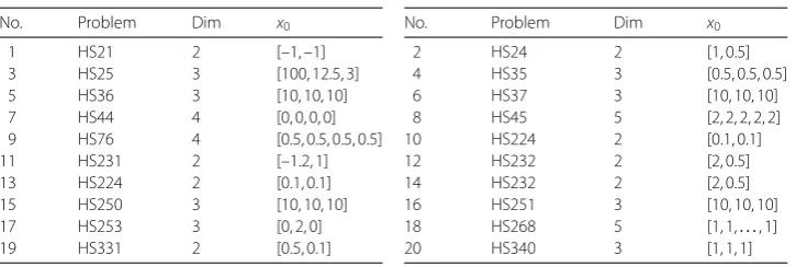
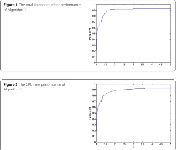
We use the tool of Dolan and Moré [17] to analyze the efficiency of the given algorithm. Figures 1 and 2 show that Algorithm 1 is feasible and has the robust property.

Furthermore we test five simple linear inequality constrained optimization problems from [16] and compare the experiment results of different trust-region radius upper bound

Figure 1The total iteration number performance of Algorithm 1

Table 2 Experiment results on linear inequality constrained optimization problems

Problem name Results

max= 4 max= 6 max= 8

n nf CPUt nf CPUt nf CPUt

HS224 2 26 5.187 23 3.35 23 3.35

HS231 2 16 2.025 18 4.018 F F

HS232 2 8 2.387 23 2.455 F F

HS250 3 12 55 17 73 16 61

HS251 3 35 3.036 32 2.022 37 2.332

max. Table 2 shows the experiment results, wherenf represents the number of function

evaluations,nis the dimension of the test problems andFmeans the algorithm terminated

in the case that the iteration number exceeds the maximum number. The CPU times of the test problems are reported. Table 2 indicates that Algorithm 1 is executable to reach

optimal point. The choice ofmax= 6 is made to enable us to carry out more gratifying

results. But the results show that the number of iterations maybe higher than any other derivative-based algorithms. The reason we think is that the derivatives of most of the test problems we chose are available and a derivative-free technique may increase the number of executions; then higher iteration numbers are necessary.

5 Conclusions

In this paper, we propose an affine-scaling derivative-free method for linear inequality constrained optimizations.

(1) This algorithm is mainly designed to solve the unavailable derivatives optimization problems in engineering. The proposed algorithm adopts interior backtracking technique and possesses the trust-region property.

(2) The global convergence is proved by using the definition of fully quadratic. It shows that the iteration points generated by the proposed algorithm could converge to the optimal points of (1). Meanwhile, we get the result that the local convergence rate of the proposed algorithm depends onpk. Ifpkbecomes the quasi-Newton step, then the sequencexkgenerated by the algorithm converges tox∗superlinearly.

(3) The preliminary numerical experiments verify the new algorithm we proposed is feasible and effective for solving unavailable-derivative linear inequality constrained optimization problems.

Acknowledgements

This work is supported by the National Science Foundation of China under Grant No. 11626037, 13th five-year Science and Technology Project of Education Department of Jilin Province under Grant No. JJKH20170036KJ, the PhD Start-up Fund of Natural Science Foundation of Beihua University and Youth Training Project Foundation of Beihua University.

Competing interests

The authors declare that they have no competing interests.

Authors’ contributions

All authors contributed equally and significantly in writing this article. All authors read and approved the final manuscript.

Author details

1_{School of Mathematics and Statistics, Beihua University, Jilin, P.R. China.}2_{School of Information Technology and Media,}

Beihua University, Jilin, P.R. China.

Publisher’s Note

Received: 17 January 2018 Accepted: 26 April 2018 References

1. Kanzow, C., Klug, A.: An interior-point affine-scaling trust-region method for semismooth equations with box constraints. Comput. Optim. Appl.37(3), 329–353 (2007)

2. Kanzow, C., Klug, A.: On affine-acaling interior-point Newton methods for nonlinear minimization with bound constraints, Comput. Optim. Appl.35(2), 177–197 (2006)

3. Heinkenschloss, M., Ulbrich, M., Ulbrich, S.: Superlinear and quadratic convergence of affine-scaling interior-point Newton methods for problems with simple bounds without strict complementarity assumption. Math. Program.

86(3), 615–635 (1999)

4. Liuzzi, G., Lucidi, S., Sciandrone, M.: Sequential penalty derivative-free methods for nonlinear constrained optimization. SIAM J. Optim.20(5), 2614–2635 (2010)

5. Coleman, T.F., Li, Y.: A trust region and affine scaling interior point method for nonconvex minimization with linear inequality constraints. Math. Program.88(1), 1–31 (1997)

6. Zhu, D.: A new affine scaling interior point algorithm for nonlinear optimization subject to linear equality and inequality constraints. J. Comput. Appl. Math.161(1), 1–25 (2003)

7. Sahu, D.R., Yao, J.C.: A generalized hybrid steepest descent method and applications. J. Nonlinear Var. Anal.1, 111–126 (2017)

8. Gibali, A.: Two simple relaxed perturbed extragradient methods for solving variational inequlities in Euclidean spaces. J. Nonlinear Var. Anal.2, 49–61 (2018)

9. Zhang, H., Conn, A.R., Scheinberg, K.: A derivative-free algorithm for least-squares minimization. SIAM J. Optim.20(6), 3555–3576 (2010)

10. Zhang, H., Conn, A.R.: On the local convergence of a derivative-free algorithm for least-squares minimization. Comput. Optim. Appl.51(2), 481–507 (2012)

11. Liuzzi, G., Lucidi, S., Rinaldi, F.: A derivative-free approach to constrained multiobjective nonsmooth optimization. SIAM J. Optim.26(4), 2744–2774 (2016)

12. Tung, L.T.: Higher-order contingent derivative of perturbation maps in multiobjective optimization. J. Nonlinear Funct. Anal.2015, 19 (2015)

13. Conn, A.R., Scheinberg, K., Vicente, L.N.: Global convergence of general derivative-free trust-region algorithms to first-and second-order critical points. SIAM J. Optim.20(1), 387–415 (2006)

14. Jing, G., Zhu, D.: An affine scaling derivative-free trust region method with interior backtracking technique for bounded-constrained nonlinear programming. J. Syst. Sci. Complex.27(3), 537–564 (2014)

15. Hock, W., Schittkowski, K.: Test Examples for Nonlinear Programming Codes. Springer, Bayreuth (1987) 16. Schittkowski, K.: More test examples for nonlinear programming codes (1987)