A robust design in hardfacing using a plasma transfer arc

DOI 10.1007/s00170-004-2265-6 O R I G I N A L A R T I C L E

Shu-Yi Tu · Ming-Der Jean · Jen-Ting Wang · Chun-Sen Wu

A robust design in hardfacing using a plasma transfer arc

Received: 4 March 2004 / Accepted: 19 May 2004 / Published online: 20 April 2005 ©Springer-Verlag London Limited 2005

Abstract This paper presents the use of the Taguchi-regression

method in developing the optimal plasma transferred arc weld-ing (PTAW) process for obtainweld-ing high hardfacweld-ing quality char-acteristics. An “optimal” process means that the best perform-ance characteristic would be produced while the least number of process parameters are involved. In the experimental tests, the surface hardening process is conducted using Cobalt-based and Nickel-based powdery metal materials together with L18 orth-ogonal arrays. The dependent variable, wear, obeys the-smaller-the-better quality characteristic, and the performance statistics, the signal-to-noise ratios (SNRs), are obtainable.

The experimental results show that the most efficient process parameters based on analysis of variance are set as follows: hard-facing material, the accelerating voltage, the powder feed rate , and the pre-heat treatment temperature. They account for almost 90% of the total variance of wear. Under the optimal setting, the average error rates for using Taguchi and Taguchi-regression methods are 7.05 and 5.50%, respectively. The outcome of the experiment indicates that predicted values of the optimal setting fit well with the actual data. The reproducibility of the optimal plasma transfer arc hardfacing is obtained from the experimen-tal data of the confirmation run. A reliable analysis based on S.-Y. Tu

Department of Mathematics, University of Michigan at Flint, Flint, MI 48502, USA M.-D. Jean (u)

Department of Electrical Engineering, Yung-Ta Institute of Technology & Commerce, Pingtung, Taiwan,

316 Chunshan Rd, Lin-Lo, Ping-Tung, Taiwan 909, R.O.C E-mail: [email protected]

Tel.: 886-8-7233733 Fax: 886-8-7236807 J.-T. Wang

Department of Mathematics, Computer Science, and Statistics, State University of New York College at Oneonta, USA C.-S. Wu

Welding Technology Section,

Metal Industries Research & Development Centre, Kaohsiung, Taiwan

the results from plasma transfer arc hardfacing conditions can be achieved through the Taguchi-regression method.

Keywords Hardfacing·Multiple linear regression·

Plasma transfer arc welding (PTAW)·Taguchi methods

1 Introduction

The plasma transfer arc (PTA) is a unique tool in the hardfacing process and has enormous applications in industry [1, 2]. PTA hardfacing can be efficiently used in almost all metals that are re-sistant to wear, such as roll surface, extruder screws, knife edges, hammer mills, tractor treads, and bucket teeth. It is also suit-able for any hardfacing application that requires minimal defect and dilution during the heating surface hardening process. On the other hand, arc welding methods such as shielded metal arc, flux core arc, and submerged arc [3, 4] are the most frequent heat-ing surface hardenheat-ing processes used in industry. These methods utilize flexible processes with low cost, but their high thickness of hard surfacing, high dilution, and poor control in melting, to some extent limit their applications.

Wear, existing normally in the form of gradual material re-moval, is an essential damage of a solid surface by relative motion with either a contacting substance or substances. It com-monly occurs on the industrial parts such as gear teeth, cams, shafts, bearings, automotive clutch plates, tools, as well as dies. A plasma transfer arc welding (PTAW) hardfacing process is a thick localized hardfacing heat treatment that is particularly useful for enhancing their surface resistance to wear.

melted zone by filler metals. It is worth pointing out that most of the studies mainly focus on the mechanical property analysis of the treated zones, but lack the process optimization.

To evaluate process performances more efficiently, Taguchi proposed a methodology that provides a simple, effective, and systematic technique to optimize process designs with better per-formance, high quality, and low cost. His work provided a fast development in many fields since the 1980s. Much work in opti-mization studies can be found in mechanical and electrical fields, but few are published in welding engineering [8–10].

Multiple regression analysis is one of the most frequently used statistical techniques, which allow one to model an appro-priate functional relationship between the response and the ex-planatory variables, as well as provide reasonable predictions of the response. Therefore, in this paper, we apply multiple regres-sion analysis to investigate the outcome for PTA surface hardfac-ing ushardfac-ing Taguchi methods. The goals for this article are to not only to present the effect of process parameters, but also develop a most effective hardfacing process using the ideas proposed.

2 PTAW hardfacing hardened processes

2.1 Plasma transfer arc welding (PTAW)

Plasma is typically a type of a gas that is heated to an extremely high temperature and then ionized so that it becomes electrically conductive. The plasma arc welding process uses this plasma to transfer an electric arc to a workpiece. The metal to be welded is first melted by the powerful heat of the arc and then fuses together. In the plasma welding torch, a Tungsten electrode is lo-cated within a copper nozzle having a small opening at the tip. A pilot arc, which is transferred to the metal to be welded, is initiated between the torch electrode and nozzle tip. By forcing the plasma gas and arc through a constricted orifice, the torch has a powerful capability in penetration and delivers a high con-centration of heat to a local area. Through the arc connecting the plasma gun and the work, PTAW generates a plasma flame whose role is to melt filler metals during the welding or hardfac-ing processes. Due to the low-power weldhardfac-ing torch and shieldhardfac-ing used in the PTAW process, argon gas generates a lower speed plasma arc and powdered filler metal by inserting gas through a constricted arc zone and creating a complicated molten hard-facing surface. In addition, the come-and-go oscillation of PTAW for hardfacing is better than automatic gas tungsten arc

weld-Symbol Control factor Level 1 Level 2 Level 3

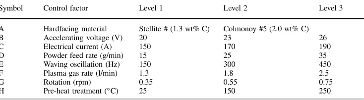
A Hardfacing material Stellite # (1.3 wt% C) Colmonoy #5 (2.0 wt% C)

B Accelerating voltage (V) 20 23 26

C Electrical current (A) 150 170 190

D Powder feed rate (g/min) 15 25 35

E Waving oscillation (Hz) 150 300 450

F Plasma gas rate (l/min) 1.3 1.8 2.5

G Rotation (rpm) 0.35 0.55 0.75

H Pre-heat treatment (◦C) 25 150 250

Table 1. Control factors and levels for L18array

Fig. 1. The plasma transfer arc welding system

ing (GTAW) with smooth, accurate weld profiles. In this study, the heating source for PTAW hardfacing experiments originates from the Nittetsu plasma transfer arc machining equipment and the process takes place in a steady powder supply granularity at the degree between 53and 150µm. From Fig. 1, it shows that the basic PTAW equipment includes a power supply for the arc, non-consumable tungsten electrode for the center, a plasma gas supply with controls, a shielding gas with controls, a water cool-ing system for the torch, and other controls to assemble all these objects. However, by programming with PTAW, the most wanted production such as engine valves, screws, and guide rollers will be able to produce any desired hardfacing patterns in the work.

2.2 Experimental materials and their characteristics

The hardfacing materials studied are the cobalt-based and the nickel-based powered alloys that consist of Stellite #1 and Col-monoy #5 in the powder metal. Tables 1 and 2 present the ex-perimental layout of the hardfacing control parameters obtained using the L18orthogonal array, and their corresponding levels. The annealing 45C carbon steel in the substrate matrix con-sists of C (0.48%), Si (0.22%), Mn (0.71%), P (0.013%) and S (0.008%). The dimensions of the specimens are 12×50× 200 mm3. PTA hardfacing is performed using Nittetsu PTA ma-chining equipment.

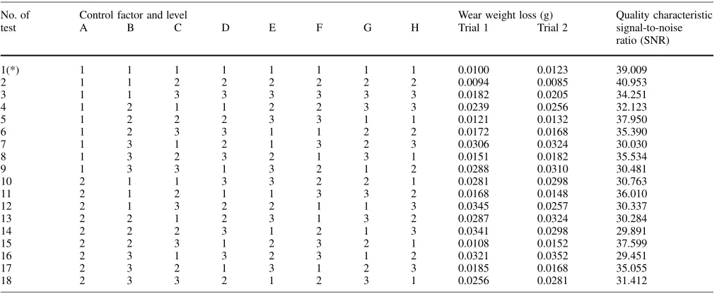
Table 2. Taguchi experimental results

No. of Control factor and level Wear weight loss (g) Quality characteristic

test A B C D E F G H Trial 1 Trial 2 signal-to-noise

ratio (SNR)

1(*) 1 1 1 1 1 1 1 1 0.0100 0.0123 39.009

2 1 1 2 2 2 2 2 2 0.0094 0.0085 40.953

3 1 1 3 3 3 3 3 3 0.0182 0.0205 34.251

4 1 2 1 1 2 2 3 3 0.0239 0.0256 32.123

5 1 2 2 2 3 3 1 1 0.0121 0.0132 37.950

6 1 2 3 3 1 1 2 2 0.0172 0.0168 35.390

7 1 3 1 2 1 3 2 3 0.0306 0.0324 30.030

8 1 3 2 3 2 1 3 1 0.0151 0.0182 35.534

9 1 3 3 1 3 2 1 2 0.0288 0.0310 30.481

10 2 1 1 3 3 2 2 1 0.0281 0.0298 30.763

11 2 1 2 1 1 3 3 2 0.0168 0.0148 36.010

12 2 1 3 2 2 1 1 3 0.0345 0.0257 30.337

13 2 2 1 2 3 1 3 2 0.0287 0.0324 30.284

14 2 2 2 3 1 2 1 3 0.0341 0.0298 29.891

15 2 2 3 1 2 3 2 1 0.0108 0.0152 37.599

16 2 3 1 3 2 3 1 2 0.0321 0.0352 29.451

17 2 3 2 1 3 1 2 3 0.0185 0.0168 35.055

18 2 3 3 2 1 2 3 1 0.0256 0.0281 31.412

(*): Initial test setting

testers as the standard in controlling experimental conditions, which include contact forces, sliding line speeds and wear slid-ing distances. The quality characteristic concerned here is the wear resistance of hardfacing-treated specimens and wear weight losses can assess it through wear tests. In general, a lower wear weight loss usually implies a better wear resistance. We perform these wear tests under conditions as follows: loading of 10 kgw, sliding speed at 1.04 m/s, a sliding distance of 500 m, and no lubricates.

2.3 PTAW hardfacing hardened properties

Hardfacing is the procedure that deposits alloys on metallic parts through welding and forms protective surface, which resists abrasion with impact, heat, corrosion, or combinations of these factors. Understanding some fundamental principles in metal-lurgy will help one to set up intelligent hardfacing procedures. The wear resistances of a hardfacing deposit depend on two vari-ables which are the analysis and cooling rate of the deposit. In this paper, we focus on analyzing a series of deposits during the welding or hardfacing processes and finding the most appropriate parameters to enhance the chance of better performance qual-ity. As for the importance of the deposits’ cooling rates, we will discuss it in future research.

3 Taguchi-regression for PTAW hardfacing

3.1 Experimental design using orthogonal arrays

The purpose of this experimental design is to optimize the PTAW hardfacing factors in addition to produce high hardfacing qual-ity. To be precise, we will apply parameter design in statistics to find the best combination of control factors. Moreover, making

use of Taguchi orthogonal arrays allows one to reduce the num-ber of necessary experimental tests. Since the orthogonal arrays are self-balanced and mutual-balanced in experimental designs, one can obtain sufficient information with only fractional facto-rial experiment. In addition, based on its good even distribution of factorial interactions over control factors, we employ a L18 array in the experimental tests.

The choices for these control factors (A-H in Table 1) in the PTAW hardfacing process are based on opinions from welding experts and the controllability of welding equipments. We select these levels for the propriety and perform 18 Taguchi experiments.

3.2 Multiple linear regression model and estimates

The multiple regression analysis is a procedure that predicts a single dependent variable by two or more independent vari-ables through a linear function. That is to say, the dependent variable Y can be predicted by a linear regression function of k independent variables X1, X2,. . ., Xk. Specifically, with a sam-ple of n observations of the dependent variable Y , the regression model can be expressed as:

Yi=β0+ k

j=1

βjXij+εi, i=1,2, . . ..,n (1)

where Yistands for the ith observation of Y , Xij denotes the ith observation of the jth independent variable, andβ0, β1, . . . , βk are the unknown regression parameters to be determined. The random errorsεi’s are assumed to be independent of each other, and follow the normal distribution with a mean of zero and a con-stant variance ofσ2. Hence, the mean of Yiis:

E(Yi)=β0+ k

j=1

Express Eq. 1 in the matrix form and yield

Y=Xβ+ε

where Y= ⎡ ⎢ ⎢ ⎣ y1 y2 : yn ⎤ ⎥ ⎥

⎦,X=

⎡ ⎢ ⎢ ⎣

1 x11. . .x1k 1 x21. . .x2k : : . . . : 1 xn1. . .xnk

⎤ ⎥ ⎥ ⎦,β=

⎡ ⎢ ⎢ ⎣ β0 β1 : βk ⎤ ⎥ ⎥ ⎦,ε=

⎡ ⎢ ⎢ ⎣ ε1 ε2 : εn ⎤ ⎥ ⎥ ⎦.

In addition, the mean of Y is:

E(Y)=Xβ.

To obtain the best prediction for Y, we apply the least squares criterion to determine the value of the regression parameter β. The least-squares estimate of the vectorβ, represented byβˆ, al-lows predicted values to be fairly close to observed values, and minimizes the sum of squares of errors (SSE), which takes the form:

SSE=

n

i=1

[Yi−E(Yi)]2=(Y−Xβ)T(Y−Xβ). (3)

Apply techniques in matrix algebra to minimize Eq. 3 and yield:

ˆ β= ⎡ ⎢ ⎢ ⎢ ⎣ ˆ β0 ˆ β1 ... ˆ βk ⎤ ⎥ ⎥ ⎥

⎦=(XTX)−1XTY (4)

provided that the matrix XT_{X is non-singular. Therefore,Y}ˆ i, de-noting the predicted value of Yi, is evaluated as:

ˆ Yi= ˆβ0+

k

j=1 ˆ

βjXij. (5)

3.3 Evaluation of signal-to-noise ratio (SNR)

Taguchi has extended the audio concept of signal-to-noise to a multivariable experimentation. The SNR formula is designed in a way such that one can select the greatest value as the optimiz-ing experimental results. However, the technique for calculatoptimiz-ing SNR varies since it depends on whether a large, small, or on target response is in question. In the PTAW hardfacing process, we want the non-negative wear weight loss to be as small as possible; therefore, a SNR formula for the-smaller-the-better re-sponse is desirable. Taguchi’s SNR formula, which takes both the average and the standard deviation into consideration, is de-rived as:

SNRi= −10 log

⎡ ⎣1

r ⎛

⎝r

j=1

Y_ij2 ⎞ ⎠ ⎤

⎦_, (6)

where SNRi represents the SNR of the ith test, Yijstands for the observed wear weight losses of the jth trial under the ith test, and r is the total number of trials under each test. In this study, we perform two repeated trials in each of the 18 hardfacing tests; therefore, r=2 and i ranges from 1 to 18. As the predicted wear weight loss for the Taguchi-regression method possesses the-smaller-the-better property, the SNR for this method can be evaluated by replacing Yij with

ˆ

Yij, which stands for the predicted wear weight loss of the jth repeated trial under the ith test obtained from the regression equations.

3.4 Analysis of variance (ANOVA)

Since we are interested in testing the effects of the control fac-tors on the response variable, wear weight loss, the ANOVA is the technique required to perform the analysis. The goal of the ANOVA is to estimate and test the effects of different treat-ments on the response variables. From the analysis, we are able to identify the most important factors in terms of the quality characteristics. The ANOVA table consists of variations (sums of squares) due to factors and random errors, degrees of free-dom, mean squares, and F ratios. The total variation, or the sum of squares (SST) of SNRs and its degrees of freedom (DOFTotal) are:

SST=

n

i=1

(SNRi− ¯SN¯R¯)2, DOFTotal=n−1, (7)

where SNRi represents the SNR of the ith test, S¯N¯R rep-¯

resents the overall mean of SNRs, and n is the number of experimental tests. The SST of SNR ratios can be partitioned into the sum of squares from each factor and the sum of squares for errors (SSE). For the J th control factor, the sum of squares, SSJ, and the corresponding degrees of freedom, DOFJ, are:

SSJ=nJ lJ

k=1

(S¯N¯R¯Jk− ¯SN¯R¯)2, DOFJ=lJ−1,J=1, . . .m,

(8)

where the S¯N¯R¯Jk is the mean of the SNRs of the J th factor measured at the kth level, lJ is the number of levels of the J th factor, nJis the total number of tests run at each level of the J th factor, and m is the number the factors. To be specific, in our study, we have,

n1=9,n2= · · · =n8=6 and l1=2,l2= · · · =l8=3.

4 Experimental results and discussion

4.1 Analysis of the experimental results

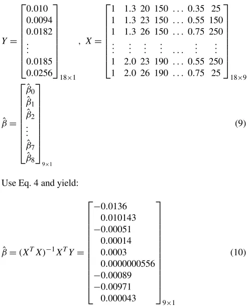
The interested quality characteristic of the PTAW hardfacing process in this study is the local wear of the hardfacing zone. Table 2 displays a complete experimental layout and their re-sultant data. Note that, in each of the tests, we carry out two repetitive trials. We use the data from the 18 various experimen-tal tests and eight independent variables to predict the minimum local wear weight losses via the multiple regression model. Ac-cording to the procedures mentioned in 3.2, we first solve the parameter vectorβˆ and then use it to obtain the predicted wear weight losses. Using data from the 1st trial, the vector Y , the matrix X, and the vectorβˆ are

Y= ⎡ ⎢ ⎢ ⎢ ⎢ ⎢ ⎢ ⎢ ⎣

0.010 0.0094 0.0182 ... 0.0185 0.0256

⎤ ⎥ ⎥ ⎥ ⎥ ⎥ ⎥ ⎥ ⎦

18×1 , X=

⎡ ⎢ ⎢ ⎢ ⎢ ⎢ ⎢ ⎢ ⎣ 1 1 1

1.3 20 150 1.3 23 150 1.3 26 150

. . . 0.35 25 . . . 0.55 150 . . . 0.75 250 ...

1 1

... ... ... 2.0 23 190 2.0 26 190

. . . ... ... . . . 0.55 250 . . . 0.75 25

⎤ ⎥ ⎥ ⎥ ⎥ ⎥ ⎥ ⎥ ⎦

18×9

ˆ β= ⎡ ⎢ ⎢ ⎢ ⎢ ⎢ ⎢ ⎢ ⎢ ⎣ ˆ β0 ˆ β1 ˆ β2 ... ˆ β7 ˆ β8 ⎤ ⎥ ⎥ ⎥ ⎥ ⎥ ⎥ ⎥ ⎥ ⎦

9×1

(9)

Use Eq. 4 and yield:

ˆ

β=(XTX)−1XTY= ⎡ ⎢ ⎢ ⎢ ⎢ ⎢ ⎢ ⎢ ⎢ ⎢ ⎢ ⎢ ⎢ ⎣

−0.0136

0.010143 −0.00051

0.00014 0.0003 0.0000000556 −0.00089 −0.00971 0.000043

⎤ ⎥ ⎥ ⎥ ⎥ ⎥ ⎥ ⎥ ⎥ ⎥ ⎥ ⎥ ⎥ ⎦

9×1

(10)

Thus, according to the observations of trial 1, the best predicted wear weightY of the PTAW hardfacing with the given values ofˆ

control variables: X1=x1,. . ., X8=x8, is:

ˆ

Y= −0.0136+0.010143X1−0.00051X2+0.00014X3 +0.0003X4+0.0000000556X5−0.00089X6

−0.00971X7+0.000043X8 (11)

Similarly, the best predicted wear weight lossY from trial 2 canˆ

be also obtained. Table 3 shows the estimated parameter vectorβˆ in the regression equations for both trials.

Table 3. Regression parameter estimates

Control factor Estimated parameter Trial 1 Trial 2

Intercept −0.0136 −0.01864

Hardfacing material (A) 0.010143 0.007825 Accelerating voltage (B) −0.00051 −0.000844 Electrical current (C) 0.000140 0.000209 Powder feed rate (D) 0.000300 0.000288 Waving oscillation (E) 5.56E-08 5.28E-06 Plasma gas rate (F) −0.00089 0.000854

Rotation (G) −0.00970 0.003166

Pre-heat temperature (H) 0.000042 0.000025

4.2 Multiple linear regression analysis of PTAW hardfacing process

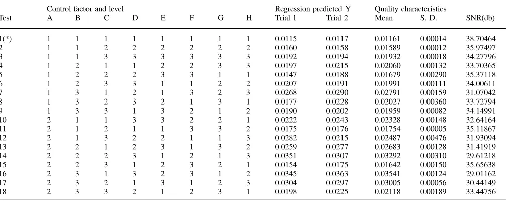
In this research, we use all the control factors as independent variables in generating a multiple linear regression model. Pre-dicted wear weight losses yielded from the least-squares regres-sion equations for both trials, and the SNRs of the 18 tests, are in Table 4. The respective coefficients of determination, R2_{, are} 0.79 and 0.74 for trials 1 and 2, which indicate that over 70% of the variation of wear is accounted for by the corresponding regression equations.

4.3 Estimated SNR effects for the quality characteristic

We evaluate the performances of each experimental test by its corresponding SNR using Eq. 6. Tables 2 and 4 provide the yielded SNRs using the Taguchi method and the Taguchi-regression method, respectively. Furthermore, the response table of the SNRs obtained from the Taguchi-regression method and the graphical representation of the response effects are shown in Table 5 and Fig. 2. It is easy to see the effects of control fac-tors and their levels from the SNRs. The range of the level-SNRs within each factor implies the significance of the factor. The larger the range, the more important the factor is. Therefore, we can identify H (pre-heat temperature) as the most significant fac-tor for the process robustness, followed by facfac-tors D (powder feed rate), B (accelerating voltage), and A (hardfacing material). They have relatively great impacts on the variability in wear. Table 5 and Fig. 2 also suggest that, for the Taguchi-regression method, the best levels for each control factor are A1, B1, C3, D1, E1, F3, G3 and H1 since they have the highest SNRs within these factors. To summarize, the best experimental treatment is set as follows: cobalt-based, accelerating voltage at 20 V, electric current at 190 A, the rate of powder feed at 15 g/min, waving os-cillation at 150 Hz, the rate of plasma gas at 2.5 l/min, the speed of rotation at 0.75 rpm, and pre-heat temperature at 25◦C.

4.4 Prediction of the optimized PTAW hardfacing process

Table 4. Taguchi-regression experimental results

Control factor and level Regression predicted Y Quality characteristics

Test A B C D E F G H Trial 1 Trial 2 Mean S. D. SNR(db)

1(*) 1 1 1 1 1 1 1 1 0.0115 0.0117 0.01161 0.00014 38.70464

2 1 1 2 2 2 2 2 2 0.0160 0.0158 0.01589 0.00012 35.97497

3 1 1 3 3 3 3 3 3 0.0192 0.0194 0.01932 0.00018 34.27796

4 1 2 1 1 2 2 3 3 0.0197 0.0215 0.02060 0.00132 33.70365

5 1 2 2 2 3 3 1 1 0.0147 0.0188 0.01679 0.00290 35.37118

6 1 2 3 3 1 1 2 2 0.0207 0.0191 0.01991 0.00111 34.00611

7 1 3 1 2 1 3 2 3 0.0268 0.0290 0.02791 0.00159 31.07042

8 1 3 2 3 2 1 3 1 0.0177 0.0228 0.02027 0.00360 33.72794

9 1 3 3 1 3 2 1 2 0.0190 0.0202 0.01959 0.00082 34.14991

10 2 1 1 3 3 2 2 1 0.0222 0.0243 0.02328 0.00148 32.64164

11 2 1 2 1 1 3 3 2 0.0175 0.0176 0.01754 0.00005 35.11867

12 2 1 3 2 2 1 1 3 0.0282 0.0215 0.02487 0.00476 31.93094

13 2 2 1 2 3 1 3 2 0.0259 0.0277 0.02683 0.00128 31.41919

14 2 2 2 3 1 2 1 3 0.0351 0.0307 0.03292 0.00310 29.61218

15 2 2 3 1 2 3 2 1 0.0154 0.0175 0.01642 0.00150 35.65638

16 2 3 1 3 2 3 1 2 0.0345 0.0363 0.03541 0.00124 29.01162

17 2 3 2 1 3 1 2 3 0.0304 0.0297 0.03005 0.00056 30.44149

18 2 3 3 2 1 2 3 1 0.0198 0.0225 0.02118 0.00189 33.44756

(*): Initial test setting

Table 5. The response table of SNRs for the Taguchi-regression method

A B C D E F G H

Level 1 34,55 34,77 32,76 34,63 33,66 33,37 33,13 34,92

Level 2 32,14 33,29 33,37 33,20 33,33 33,25 33,30 33,28

Level 3 N/A 31,97 33,91 32,21 33,05 33,42 33,62 31,84

Effect 2,41 2,80 1,15 2,42 0,61 0,16 0,49 3,09

estimate their SNRs through the additivity law of the linearity of the PTAW hardfacing process. Hence, the formula is as follows:

SNROptimal= ¯SN¯R¯+ m

J=1

(SNRJ− ¯SN¯R¯) (12)

where SNROptimalis the estimated SNR of the optimal setting,

SNRJis the highest level-SNR of the jth factor,S¯N¯R is the over-¯ all average of SNRs, and m is the number of factors. Based on Eq. 5, the predicted SNRs for the optimal settings from both the Taguchi method and the Taguchi-regression method are 44.3200 and 41.5204, respectively.

4.5 Verification experiments

The confirmation experiments for the optimal settings using both methods are performed for the verification purpose. We also use test 1 as the initial test to compare with the optimal tests for both methods. The experimental results and comparisons with the pre-dicted SNRs are listed in Tables 6 and 7. Experimental results show that the actual gain of SNR is 2.1347 db in the Taguchi method and 3.9858 db in the Taguchi-regression method. They also show that the latter method produces an SNR that is closer to the prediction. Undoubtedly, the Taguchi-regression method

Fig. 2. The SNR response graph for the Taguchi-regression method

is superior to the Taguchi method since it yields higher SNRs, which is equivalent to meaning better quality. These predicted gains not only confirm excellent additive or reproducibility but also provides us sufficient confidence in the factorial effects we select as important. It is clear in Table 7 that the optimal setting in wear weight loss by the Taguchi-regression method approach the confirmation run better than the Taguchi method. In add-ition, Taguchi-regression method results in the lower standard deviations for the whole tests, which indicates a significant im-provement in the process robustness. Furthermore, the results of confirmation runs of the optimal tests for both methods are given in Table 6. The SNR of the confirmation run of the optimal set-ting from the Taguchi method is 41.1432 db, while the SNR is 42.6904 db from the Taguchi-regression method, which is the largest among all the experiments. The corresponding average weight loss from the optimal setting is 0.00734 g, which is the lowest and actually is much lower than the initial setting.

4.6 ANOVA using Taguchi-regression method

Table 6. Verification experiments

Test Control factors and level Quality characteristics Confirmation

A B C D E F G H Trial 1 Trial 2 Mean S. D. SNR (db)

Optimal 1 1 2 1 2 1 2 1 0.0089 0.0086 0.0087 0.0002474 41.1432

Taguchi setting

Optimal 1 1 3 1 1 3 3 1 0.0065 0.0072 0.0073 0.0001770 42.6904

Taguchi regression setting

Test Taguchi-regression Taguchi Taguchi-regression Taguchi prediction prediction confirmation confirmation

(db) (db) (db) (db)

Initial setting 38.3813 39.8561 38.7046 39.0085

Optimal setting 41.5204 44.3200 42.6904 41.1432

Gain 3.2191 4.4639 3.9858 2.1347

Table 7. Comparisons between the initial test and the optimal test

to identify the important factors for the quality characteristic. Therefore, we can control those selected factors more carefully during the process so to make sure stable and high quality prod-ucts can be produced.

The ANOVA results for the Taguchi-regression are shown in Table 8. We can identify that factors H, A, B, and D are the most significant processing parameters, in descending impor-tance order. Their individual contribution percentages are well above 15% and the whole accounts for about 90% of the total variance. Clearly, conclusions drawn from the ANOVA coincide with those reflected in Table 5 and Fig. 2.

4.7 Comparisons between Taguchi and Taguchi-regression methods

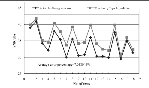
In order to obtain a fair and systematical comparison between the Taguchi and Taguchi-regression methods, we use the same set-tings for each process factors in the experimental tests and check the wear loss using both methods. The predictions and com-parisons to the actual wear loss shown in Figures 3 and 4 both indicate that predicted and actual values are quite close using

Table 8. ANOVA table for the Taguchi-regression method

Source of variation Sum of squares Degrees of freedom Mean of squares F ratio Pure sum of square Percentage contribution

A 26.1777 1 26.1777 50.303 25.6573 24.9108

B 23.5453 2 11.7727 22.622 22.5045 21.8498

C 3.9941 2 1.9970 3.838 2.9533 2.8674

D 17.7055 2 8.8527 17.011 16.6647 16.1799

E 1.1169 2 0.5585 1.073 0.0761 0.0739

F 0.0844 2 0.0422 0.081 −0.9564 −0.9285

G 0.7300 2 0.3650 0.701 −0.3108 −0.3017

H 28.6017 2 14.3008 27.481 27.5609 26.7591

Error 1.0408 2 0.5204 1.000 8.5894

Total 102.9964 17 100

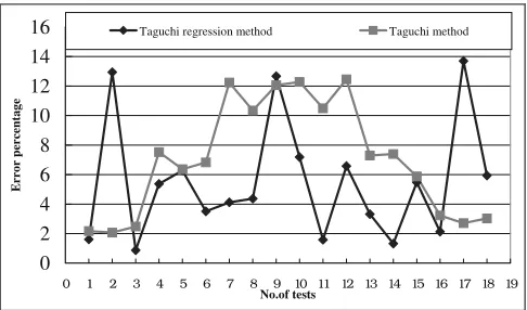
both methods, which implies that they both provide satisfac-tory predictions. However, with a closer inspection, we can find that the Taguchi-regression provides a better fit than the Taguchi method. Figure 5 plots the error percentages between the pre-dicted and the actual data for both methods used for the

Fig. 4. Comparison between Taguchi Regression predictions and actual values

Fig. 5. Error percentages for Taguchi and Taguchi-regression methods

ments. It is quite clear that the Taguchi-regression method gener-ates less error in predicting wear weight losses than the Taguchi method in most tests. To be more precise, the average error of the prediction is 5.50% in Taguchi-regression and 7.05% in the Taguchi method. Therefore, the Taguchi-Regression method is a more accurate technique for predicting the wear loss in PTAW hardfacing.

5 Conclusions

This article presents the use of the Taguchi-regression in de-veloping a robust, high speed, and high quality PTAW hard-facing process. Through proper system model simulations, quality characteristics in the hardfacing process can be opti-mized. Comparing the experimental results between the Taguchi and the Taguchi-regression methods, we have the following conclusions:

1. The most important factors that affect the wear weight loss are the hardfacing materials, accelerating voltages, powder feed rates, and pre-heat treatments. These factors account for about 90% of the total variance.

2. For both methods, the following settings are predicted to yield the best result:

For the Taguchi method:

Factor A – level 1, Factor B – level 1, Factor C – level 2, Factor D – level 1,

Factor E – level 2, Factor F – level 1, Factor G – level 2, Factor H – level 1.

For the Taguchi-regression method:

Factor A – level 1, Factor B – level 1, Factor C – level 3, Factor D – level 1,

Factor E – level 1, Factor F – level 3, Factor G – level 3, Factor H – level 1.

3. Comparing the increases in SNRs, using the Taguchi and the Taguchi-regression methods, we have the predicted gain of 4.4639 db and 3.9858 db, respectively, while gains of 2.1347 db and 3.2191 db through confirmation experiments, respectively. It shows that the Taguchi-regression method performs better than the Taguchi method in reproducibility. 4. The average error of 7.05% db in the Taguchi method and

5.50% in the Taguchi-regression method for the optimal set-ting, which makes process robustness, the Taguchi method has higher error than the Taguchi-regression method. 5. From the experimental results, both methods show a good

prediction for the actual values; however, the Taguchi-regression method has a better fit.

References

1. Sharples RV (1985) The plasma transferred arc weld surfacing process. The Welding Institute, USA

2. Jeffus L (1999) Welding: principles and applications, 4th ed. Interna-tional Thomson Publishing, Albany, NY

3. Devletian JH (1978) Weldability of grey iron using fluxless grey iron electrodes for SMAW. Weld J 57:183–188

4. Kelly TJ Welding ductile iron with Ni-Fe-Mn filler metals. Weld J, 64:79–85

5. Mathur AK (1985) Laser heat of cast iron. Trans ASME 107:200–207 6. Ishida T A microstructural study of local melting gray cast iron with

a stationary plasma arc. Weld J 64:232–241

7. Chakrabarti AK A metallographic study of transformation in remelted ductile iron. Indian Met 35:391–395

8. Vijaya M, Krishna R, Prabhakar O, Shankar NG (1996) Simultaneous op-timization of flame spraying process parameters for high quality molyb-denum coatings using Taguchi methods. Surf Coat Technol 79:276–288 9. Black JT, Jiang BC (1990) Robot process capability study using

Taguchi methods. Manuf Rev 3:106–114