On LQP alternating direction method for solving variational inequality problems with separable structure

R E S E A R C H

Open Access

On LQP alternating direction method for

solving variational inequality problems with

separable structure

Abdellah Bnouhachem

*_{Correspondence:}

[email protected]

School of Management Science and Engineering, Nanjing University, Nanjing, 210093, P.R. China ENSA, Ibn Zohr University, Agadir, BP 1136, Morocco

Abstract

In this paper, we proposed a logarithmic-quadratic proximal alternating direction method for structured variational inequalities. The new iterate is obtained by a convex combination of the previous point and the one generated by a projection-type method along a new descent direction. Global convergence of the new method is proved under certain assumptions. We also reported some numerical results to illustrate the efficiency of the proposed method.

MSC: 90C33; 49J40

Keywords: variational inequalities; monotone operator; logarithmic-quadratic proximal method; projection method; alternating direction method

1 Introduction

The problem we are concerned with in this paper is for the following variational inequal-ities: findu∈such that

u–uTF(u)≥, ∀u∈, (.)

with

u=

x y

, F(u) =

f(x) g(y)

and

=(x,y)|x∈Rn₊₊,y∈Rm₊₊,Ax+By=b,

(.)

whereA∈Rl×n_,B∈Rl×m_{are given matrices,b∈R}l_{is a given vector, andf:R}n

++→Rn,

g:Rm

++→Rmare given monotone operators. Studies and applications of such problems

can be found in [–]. By attaching a Lagrange multiplier vectorλ∈Rl to the linear constraintsAx+By=b, the problem (.)-(.) can be explained in terms of findingw∈W such that

w–wTQ(w)≥, ∀w∈W, (.)

where

w=

⎛ ⎜ ⎝

x y

λ ⎞ ⎟

⎠, Q(w) =

⎛ ⎜ ⎝

f(x) –AT_λ g(y) –BT_λ Ax+By–b

⎞ ⎟

⎠, W=Rn₊₊×Rm₊₊×Rl. (.)

The problem (.)-(.) is referred to as SVI (structured variational inequalities). The alternating direction method (ADM) is a powerful method for solving the struc-tured problem (.)-(.), since it decomposes the original problems into a series subprob-lems with lower scale, originally proposed by Gabay and Mercier [] and Gabay []. The classical proximal alternating direction method (PADM) [–] is an effective numeri-cal approach for solving variational inequalities with a separable structure. To make the PADM more efficient and practical, Heet al.[] proposed a modified PADM as follows. For given (xk,yk,λk)∈Rn₊₊×R₊₊m ×Rl, the new iterative (xk+,yk+,λk+) is obtained via the following steps.

Step . Solve the following system of nonlinear equations to obtainxk+_:

x–xk+Tfxk+–ATλk–HkAxk++Byk–b+Rkxk+–xk

≥, ∀x∈Rn₊₊. (.)

Step . Solve the following system of nonlinear equations to obtainyk+_:

y–yk+Tgyk+–BTλk–HkAxk++Byk+–b+Skyk+–yk

≥, ∀y∈Rm₊₊. (.)

Step . Updateλkvia

λk+=λk–HkAxk++Byk+–b. (.)

Yuan and Li [] have developed a logarithmic-quadratic proximal (LQP)-based de-composition method by applying the LQP terms to regularize the ADM subproblems, by substituting in the alternating directions method (.)-(.) the term R(x–xk) and S(y–yk_{) byR[(x–x}k_{) +μ(x}k_–X

kx–)] andS[(y–yk) +μ(yk–Yky–)], respectively. The new iterative (xk+_,yk+_,λk+_{) in [] is obtained via the following procedure: From a given}

wk_{= (x}k_,yk_,λk_)∈Rn

++×Rm++×Rlandμ∈(, ), (xk+,yk+,λk+) is obtained via solving

the following system:

f(x) –ATλk–HAx+Byk–b+Rx–xk+μxk–X_kx–= ,

g(y) –BTλk–HAxk++By–b+Sy–yk+μyk–Y_ky–= ,

λk+=λk–HAxk_+Byk_–b.

the previous point and the one generated by a projection-type method along this descent direction.

In the present paper, inspired by the above cited works and by the recent works going in this direction, we proposed a new LQP-based prediction-correction method; the new iterate is obtained by a convex combination of the previous point and the one generated by a projection-type method along another descent direction. Under the same conditions as those in [], we prove the global convergence of the proposed algorithm. It is proved theoretically that the lower bound of the progress obtained by the proposed method is greater than that by Li’s method []. The effectiveness and superiority of the proposed method is verified by our preliminary numerical experiments.

2 The proposed method

In this section, we recall some basic definitions and properties, which will be frequently used in our later analysis. Some useful results proved already in the literature are also summarized. The first lemma provides some basic properties of projection onto.

Lemma . Let G be a symmetry positive definite matrix andbe a nonempty closed

convex subset of Rl,we denote P,G(·)as the projection under the G-norm,i.e.,

P,G(v) =argmin

v–uG|u∈

.

Then we have the following inequalities:

z–P,G[z]

T

GP,G[z] –v

≥, ∀z∈Rl,v∈; (.)

P,G[u] –P,G[v]_G≤ u–vG, ∀u,v∈Rl; (.)

u–P,G[z]_G≤ z–uG–z–P,G[z]_G, ∀z∈Rl,u∈. (.)

In course we always make the following standard assumptions.

Assumption A f(x) is monotone with respect toRn

++andg(y) is monotone with respect

toRm

++.

Assumption B The solution set of SVI, denoted byW∗, is nonempty.

Now, we suggest and consider the new LQP alternating direction method (LQP-ADM) for solving SVI as follows.

Prediction step: For a givenwk_{= (x}k_,yk_,λk_)∈Rn

++×Rm++×Rl, andμ∈(, ), the

pre-dictorw˜k_{= (x˜}k_,y˜k_,λ˜k_)∈Rn

++×Rm++×Rlis obtained via solving the following system:

f(x) –ATλk–HAx+Byk–b+Rx–xk+μxk–X_kx–= , (.a)

g(y) –BTλk–H(Ax+By–b)+Sy–yk+μyk–Y_ky–= , (.b) ˜

λk=λk–HAx˜k+B˜yk–b. (.c)

Correction step: The new iteratewk+_(α

k) = (xk+,yk+,λk+) is given by

wk+(αk) = ( –σ)wk+σPW

where

αk=

ϕk

wk_–w˜k

G

, (.)

ϕk:=wk–w˜k



M+

λk–λ˜kTByk–B˜yk, (.)

dwk,w˜k=

⎛ ⎜ ⎝

f(x˜k_{) –A}T_λ˜k_+AT_HB(yk_–y˜k₎ g(y˜k_{) –B}T_λ˜k_+BT_HB(yk_–y˜k₎

Ax˜k_+B˜yk_–b

⎞ ⎟ ⎠

and

G=

⎛ ⎜ ⎝

( +μ)R  

 ( +μ)S+BT_{HB }

  H–

⎞ ⎟

⎠, M=

⎛ ⎜ ⎝

R  

 S+BT_{HB }

  H–

⎞ ⎟ ⎠.

Remark . Ifxk+_=x˜k_,yk+_=˜yk_andλk+_=λ˜k_{in (.a), (.b), and (.c), respectively,} we obtain the method proposed in [].

We need the following result in the convergence analysis of the proposed method.

Lemma .[] Let q(u)∈Rnbe a monotone mapping of u with respect toRn+and R∈

Rn×n_{be positive definite diagonal matrix.For given u}k_{> ,if we let U}

k:=diag(uk,uk, . . . ,ukn) and u–_{be an n-vector whose jth element is/u}

j,then the equation

q(u) +Ru–uk+μuk–U_ku–=  (.)

has a unique positive solution u.Moreover,for any v≥,we have

(v–u)Tq(u)≥ +μ 

u–v_R–uk–v_R+ –μ  u

k_–u

R. (.)

In the next theorem we show thatαkis lower bounded away from zero and it is one of the keys to prove the global convergence results.

Theorem . For given wk_∈Rn

++×Rm++×Rl,letw˜kbe generated by(.a)-(.c),then

we have the following:

ϕk≥  Ax˜

k_+Byk_–b H+w

k_–w˜k G

(.)

and

αk≥ 

. (.)

Proof It follows from (.) that

ϕk=wk–w˜k



M+

λk–λ˜kTByk–By˜k

=xk–x˜k_R+yk–y˜k_S+Byk–By˜k_H+λk–λ˜k_H–

Using (.c), we have

λk–λ˜kTByk–By˜k+ By

k_–By˜k

H+λ k_–λ˜k

H–

=Ax˜k+By˜k–bTHByk–By˜k+ By

k_–By˜k H+Ax˜

k_+By˜k_–b H

= Ax˜

k_+Byk_–b

H. (.)

Substituting (.) into (.), we get

ϕk =  Ax˜

k_+Byk_–b H+By

k_–By˜k H+λ

k_–λ˜k H–

+xk–x˜k_R+yk–y˜k_S

=  Ax˜

k_+Byk_–b

H+w k_–w˜k

G+ ( –μ)x k_–x˜k

R+ ( –μ)y k_–y˜k

S

≥  Ax˜

k_+Byk_–b H+w

k_–w˜k G

.

Therefore, it follows from (.) and (.) that

αk≥  

and this completes the proof.

3 Basic results

In this section, we prove some basic properties, which will be used to establish the suffi-cient and necessary conditions for the convergence of the proposed method. The follow-ing results are due to applyfollow-ing Lemma . to the LQP systems in prediction step of the proposed method.

Lemma . For given wk= (xk,yk,λk)∈R₊₊n ×Rm₊₊×Rl,letw˜kbe generated by(.a) -(.c).Then for any w∗= (x∗,y∗,λ∗)∈W∗,we have

wk–w∗TGwk–w˜k≥ϕk. (.)

Proof Applying Lemma . to (.a) (by settinguk_=xk_,u=x˜k_,v=x∗_{in (.)) and}

q(u) =fx˜k–ATλk–HAx˜k+Byk–b,

we get

x∗–x˜kT_fx˜k_–AT_λk_–HAx˜k_+Byk_–b

≥ +μ  x˜

k_–x∗

R–x k_–x∗

R

+ –μ  x

k_–x˜k

R. (.)

Recall

x∗–x˜kTRxk–x˜k= x˜

k_–x∗ R–x

k_–x∗ R

+ x

k_–x˜k

Adding (.) and (.), we obtain

x∗–x˜kT( +μ)Rxk–x˜k–fx˜k+ATλ˜k–ATHByk–˜yk≤μxk–x˜k_R. (.)

Similarly, applying Lemma . to (.b), substitutinguk_=yk_,u=˜yk_,v=y∗_{, and replacing} R,nwithS,m, respectively, in (.) and

q(u) =gy˜k–BTλk–HAx˜k+B˜yk–b,

we get

y∗–y˜kTgy˜k–BTλk–HAx˜k+By˜k–b

≥ +μ  y˜

k_–y∗

S–y k_–y∗

S

+ –μ  y

k_–y˜k

S. (.)

Recall

y∗–y˜kTSyk–y˜k= y˜

k_–y∗ S–y

k_–y∗ S

+ y

k_–y˜k

S. (.)

Adding (.) and (.), we have

y∗–y˜kT( +μ)Syk–˜yk–gy˜k+BTλ˜k≤μyk–y˜k_S. (.)

Since (x∗,y∗,λ∗) is a solution of SVI,x˜k_∈Rn

++andy˜k∈Rm++, we have

˜

xk–x∗Tfx∗–ATλ∗≥,

˜

yk–y∗Tgy∗–BTλ∗≥

and

Ax∗+By∗–b= .

Using the monotonicity off andg, we obtain

⎛ ⎜ ⎝ ˜

xk_–x∗ ˜

yk–y∗

˜ λk–λ∗

⎞ ⎟ ⎠ T⎛ ⎜ ⎝

f(x˜k_{) –A}T_λ˜k g(y˜k) –BTλ˜k

Ax˜k+By˜k–b

⎞ ⎟ ⎠≥ ⎛ ⎜ ⎝ ˜

xk_–x∗ ˜

yk–y∗

˜ λk–λ∗

⎞ ⎟ ⎠ T⎛ ⎜ ⎝

f(x∗) –AT_λ∗

g(y∗) –BTλ∗

Ax∗+By∗–b

⎞ ⎟

⎠≥. (.)

Adding (.), (.), and (.), we get

w∗–w˜kTGwk–w˜k=x∗–x˜kT( +μ)Rxk–x˜k

+y∗–y˜kT( +μ)Syk–˜yk+BTHByk–y˜k

+λ∗–λ˜kTAx˜k+By˜k_–b

+y∗–y˜kTBTHByk–y˜k+μyk–˜yk_S

=μxk–x˜k_R–Ax˜k+By˜k–bTHByk–y˜k+μyk–y˜k_S

=μxk–x˜k_R–λk–λ˜kTByk–By˜k+μyk–y˜k_S, (.)

where the last equality follows from (.c). It follows from (.) that

wk–w∗TGwk–w˜k≥wk–w˜k_G–μxk–x˜k_R–μyk–˜yk_S

+λk–λ˜kTByk–B˜yk

=xk–x˜k_R+yk–y˜k_S+Byk–By˜k_H+λk–λ˜k_H–

+λk–λ˜kTByk–B˜yk.

Using the definition ofϕkthe assertion of this lemma is proved.

Theorem . Let w∗∈W∗,wk+_(α

k)be defined by(.)and

(αk) :=wk–w∗



G–w k+_(α

k) –w∗



G, (.)

then we have

(αk)≥σwk–wk∗–αk

wk–w˜k_G+ αkϕk–αkwk–w˜k



G

, (.)

where

wk_∗=xk_∗,yk_∗,λk_∗:=P_Wwk–αkG–dwk,w˜k. (.)

Proof Similarly as in (.) and (.), we have

xk_∗–x˜kT( +μ)Rxk–x˜k–fx˜k+ATλ˜k–ATHByk–˜yk≤μxk–x˜k_R (.)

and

yk_∗–y˜kT( +μ)Syk–˜yk–gy˜k+BTλ˜k–BTHByk–y˜k+BTHByk–y˜k

≤μyk–y˜k_S. (.)

It follows from (.) and (.) that

⎛ ⎜ ⎝

xk

∗–x˜k

yk

∗–˜yk λk_∗–λ˜k

⎞ ⎟ ⎠

T⎛

⎜ ⎝

( +μ)R(xk_–x˜k_{) –f(x˜}k_{) +A}T_λ˜k_–AT_HB(yk_–y˜k₎ (( +μ)S+BT_HB)(yk_–˜yk_{) –g(y˜}k_{) +B}T_λ˜k_–BT_HB(yk_–y˜k₎

H–(λk–λ˜k) – (Ax˜k+By˜k–b)

⎞ ⎟ ⎠

≤μxk–x˜k_R+μyk–˜yk_S,

which implies

αk

wk_∗–w˜kTGwk–w˜k–dwk,w˜k– αkμxk–x˜k



R– αkμy k_–y˜k

Sincew∗∈W∗andwk

∗=PW[wk_–αkG–_d(wk_,w˜k_{)], it follows from (.) that}

wk_∗–w∗_G≤wk–αkG–dwk,w˜k–w∗_G–wk–αkG–dwk,w˜k–wk_∗_G. (.)

From (.), we get

wk+(αk) –w∗_G=( –σ)

wk–w∗+σwk_∗–w∗_G

= ( –σ)wk–w∗_G+σwk_∗–w∗_G

+ σ( –σ)wk–w∗TGwk_∗–w∗.

Using the following identity:

(a+b)TGb=a+b_G–a_G+b_G

fora=wk_–wk

∗,b=wk∗–w∗and (.), we obtain

wk+(αk) –w∗_G = ( –σ)wk–w∗_G+σwk∗–w∗G+σ( –σ)w k_–w∗

G

–wk–wk_∗_G+wk_∗–w∗_G

= ( –σ)wk–w∗_G+σwk_∗–w∗_G–σ( –σ)wk–wk_∗_G

≤( –σ)wk–w∗_G+σwk–αkG–dwk,w˜k–w∗_G

–σwk–αkG–dwk,w˜k–wk_∗_G–σ( –σ)wk–wk_∗_G. (.)

Using the definition of(αk) and (.), we get

(αk)≥σwk–wk∗G+ σ αk

wk_∗–wkTdwk,w˜k

+ σ αk

wk–w∗Tdwk,w˜k. (.)

Using the monotonicity off andg, we obtain

⎛ ⎜ ⎝ ˜

xk_–x∗ ˜

yk–y∗

˜ λk_–λ∗

⎞ ⎟ ⎠

T⎛

⎜ ⎝

f(x˜k_{) –A}T_λ˜k g(y˜k) –BTλ˜k

Ax˜k_+By˜k_–b

⎞ ⎟ ⎠≥

⎛ ⎜ ⎝ ˜

xk_–x∗ ˜

yk–y∗

˜ λk_–λ∗

⎞ ⎟ ⎠

T⎛

⎜ ⎝

f(x∗) –AT_λ∗

g(y∗) –BTλ∗

Ax∗+By∗–b

⎞ ⎟ ⎠≥

and consequently

˜

wk–w∗Tdwk,w˜k≥w˜k–w∗T

⎛ ⎜ ⎝

AT_HB(yk_–y˜k₎ BT_HB(yk_–y˜k₎



⎞ ⎟ ⎠

=Ax˜k+Bx˜k–bTHByk–˜yk

=λk–λ˜kTByk–y˜k

and it follows that

Applying (.) to the last term in the right side of (.), we obtain

(αk)≥σwk–wk∗G+ σ αk

wk_∗–wkTdwk,w˜k

+ σ αk

wk–w˜kTdwk,w˜k+λk–λ˜kTByk–˜yk

=σwk–wk_∗_G+ αk

wk_∗–w˜kTdwk,w˜k

+ αk

λk–λ˜kTByk–y˜k. (.)

Adding (.) (multiplied byσ) to (.), we get

(αk)≥σwk–wk_∗_G+ αk

wk_∗–w˜kTGwk–w˜k– αkμxk–x˜k_R

– αkμyk–y˜k_S+ αk

λk–λ˜kTByk–y˜k

=σwk–wk_∗–αk

wk–w˜k_G –α_kwk–w˜k_G+ αkwk–w˜k_G

– αkμxk–x˜k_R– αkμyk–y˜k_S+ αk

λk–λ˜kTByk–y˜k

and using the notation ofϕkin (.), the theorem is proved.

From the computational point of view, a relaxation factorγ ∈(, ) is preferable in the correction. We are now at the position to prove the contractive property of the iterative sequence.

Theorem . Let w∗∈W∗ be a solution of SVI and let wk+(γ αk)be generated by(.). Then wkandw˜kare bounded,and

wk+(γ αk) –w∗



G≤w k_–w∗

G–cw k_–w˜k

G, (.)

where

c:=σ γ( –γ)  > .

Proof It follows from (.), (.), and (.) that

_wk+_{(γ α}

k) –w∗



G≤w k_–w∗

G–σ

γ αkϕk–γαkwk–w˜k



G

=wk_–w∗

G–γ( –γ)αkσ ϕk

≤wk–w∗_G–σ γ( –γ)  Ax˜

k_+Byk_–b

H+w k_–w˜k

G

.

Sinceγ∈(, ) we have

wk+–w∗≤wk–w∗≤ · · · ≤w–w∗

and thus{wk_{}is a bounded sequence.} It follows from (.) that

∞

k=

which means that

lim

k→∞w

k_–w˜k

G= . (.)

Since{wk_{}is a bounded sequence, we conclude that{ ˜w}k_{}is also bounded.}

4 Convergence of the proposed method

In this section, we prove the global convergence of the proposed method. The following results can be proved by using the technique of Lemma . and Theorem . in [].

Lemma . For given wk_{= (x}k_,yk_,λk_)∈Rn

++×Rm++×Rl,letw˜k= (x˜k,y˜k,λ˜k)be generated

by(.a)-(.c).Then for any w= (x,y,λ)∈W,we have

x–x˜kTfx˜k–ATλ˜k+ATHByk–y˜k≥xk–x˜kTR( +μ)x–μxk+x˜k (.)

and

y–y˜kTg˜yk–BTλ˜k≥yk–y˜kTS( +μ)y–μyk+y˜k. (.)

Proof Applying Lemma . to prediction step of LQP-ADM (by settinguk_=xk_,u=x˜k_, q(u) =f(x˜k_{) –A}T_λ˜k_+AT_HB(yk_–y˜k_{) andv=xin (.)), it follows that}

x–x˜kTfx˜k–ATλ˜k+ATHByk–y˜k

≥ +μ  x˜

k_–x R–x

k_–x R

+ –μ  x

k_–x˜k R.

By a simple manipulation, we have

 +μ

 x˜ k_–x

R–x k_–x

R

+ –μ  x

k_–x˜k

R

= ( +μ)xTRxk– ( +μ)xTRx˜k– ( –μ)x˜kTRxk–μxk_R+x˜k_R

= ( +μ)xTRxk–x˜k–xk–x˜kTRμxk+x˜k

=xk_–x˜kT_{R( +μ)x–μx}k_+x˜k_,

and the assertion (.) is proved. Similarly we can prove the assertion (.).

Now, we are ready to prove the convergence of the proposed method.

Theorem . The sequence{wk_{}generated by the proposed method converges to some w}∞ which is a solution of SVI.

Proof It follows from (.) that

lim

k→∞x

k_–x˜k

R= , _klim_→∞y k_–y˜k

and

lim

k→∞

λk–λ˜k

H–= lim

k→∞

Ax˜k+By˜k–b_H= . (.)

Moreover, (.) and (.) imply that

x–x˜kTfx˜k–ATλ˜k≥xk–x˜kTR( +μ)x–μxk+x˜k–x–x˜kTATHByk–y˜k

and

y–y˜kTg˜yk–BTλ˜k≥yk–y˜kTS( +μ)y–μyk+y˜k.

We deduce from (.) that

limk→∞(x–x˜k)T{f(x˜k) –ATλ˜k} ≥, ∀x∈Rn

++, lim_k→∞(y–y˜k₎T_{g(y˜k_{) –B}T_λ˜k_{} ≥, ∀y∈R}m

++.

(.)

Since{wk_{}is bounded, so it has at least one cluster point. Letw}∞_{be a cluster point of{w}k_} and the subsequence{wkj}_{converges tow}∞_{. It follows from (.) and (.) that}

⎧ ⎪ ⎨ ⎪ ⎩

limj→∞(x–xkj)T{f(xkj) –ATλkj} ≥, ∀x∈Rn++, limj→∞(y–ykj)T{g(ykj) –BTλkj} ≥, ∀y∈Rm++, lim_j→∞(Axkj_+Bykj_{–b) = .}

Consequently

⎧ ⎪ ⎨ ⎪ ⎩

(x–x∞)T_{f(x∞_{) –A}T_λ∞_{} ≥, ∀x∈R}n

++,

(y–y∞)T{g(y∞) –BTλ∞} ≥, ∀y∈Rm₊₊, Ax∞+By∞–b= ,

which means thatw∞is a solution of SVI.

Now we prove that the sequence{wk_{}converges tow}∞_{. Since}

lim

k→∞

wk–w˜k_G=  and w˜kj→_w∞

for any > , there exists anl>  such that

w_˜kl_–w∞_<

 and w

kl_–w˜kl_<

. (.)

Therefore, for anyk≥kl, it follows from (.) and (.) that

wk–w∞≤wkl_–w∞≤_wkl_–w˜kl_+w˜kl_–w∞_{< .}

5 Comparison Let

wk_I+(αk) :=PW

wk–αkG–dwk,w˜k (.)

and

wk_II+(αk) :=PW

wk–αk

wk–w˜k (.)

represent the new iterates generated by the algorithm presented in this paper and Li’s algorithm in [], respectively, whereσ= . Let

I(αk) :=wk–w∗



G–w k+

I (αk) –w∗



G

and

II(αk) :=wk–w∗_G–wkII+(αk) –w∗_G

measure the progresses made by the new iterates, respectively. From (.), we have

I(αk)≥qI(αk) :=wk–wkI+(αk) –αk

wk–w˜k_G+ αkϕk–αkwk–w˜k



G.

Theorem . of [] indicates that

II(αk)≥qII(αk) := αkϕk–αkwk–w˜k



G.

Note that the optimal step sizes used in both methods are identical. It is easy to prove that

qI(αk)≥qII(αk). (.)

Inequality (.) shows theoretically that the proposed method is expected to make more progress than that in [] at each iteration, and so it explains theoretically that the pro-posed method outperforms the method in [].

6 Preliminary computational results

In this section, we report some numerical results of the proposed method, we consider the following optimization problem with matrix variables:

min



X–C



FX∈Sn+

, (.)

where · Fis the matrix Fröbenius norm,i.e.,CF= (ni= n

j=|Cij|)/,

Sn₊=H∈Rn×n|HT=H,H.

Note that the matrix Fröbenius norm is induced by the inner product

Note that the problem (.) is equivalent to the following:

min

X–C

₊

Y–C



s.t.X–Y= , (.)

X,Y∈Sn₊,

which is equivalent to the following variational inequality: to findu∗= (X∗,Y∗,Z∗)∈= Sn

+×Sn+×Rn×nsuch that ⎧

⎪ ⎨ ⎪ ⎩

X–X∗, (X∗–C) –Z∗ ≥,

Y–Y∗, (Y∗–C) +Z∗ ≥, ∀u= (X,Y,Z)∈, X∗–Y∗= .

(.)

The problem (.) is a special case of (.)-(.) with matrix variables where A=In×n, B= –In×n,b= ,f(X) =X–C,g(Y) =Y–CandW=S+n×Sn+×Rn×n.

For simplification, we takeR=rIn×n,S=sIn×nandH=In×nwherer>  ands>  are scalars. In all tests we takeμ= .,C=rand(n) and (X,Y,Z) = (In×n,In×n, n×n) as the initial point in the test. The iteration is stopped as soon as

maxXk–X˜k,Yk–Y˜k,Zk–Z˜k≤–.

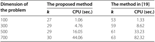
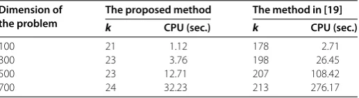
All codes were written in Matlab; we compare the proposed method with that in []. The iteration numbers denoted byk, and the computational time for the problem (.) with different dimensions are given in Tables -.

Tables - show that the proposed method is more flexible and efficient. Moreover, it demonstrates computationally that the new method is more effective than the method presented in [] in the sense that the new method needs fewer iterations and less com-putational time, which clearly illustrates its efficiency and thus justifies the theoretical assertions.

Table 1 Numerical results for the problem (6.1) withr=s= 0.8

Dimension of the problem

The proposed method The method in [19]

k CPU (sec.) k CPU (sec.)

100 29 1.17 46 1.31

300 31 5.07 50 7.43

500 32 17.92 52 27.67

700 32 42.65 54 71.13

Table 2 Numerical results for the problem (6.1) withr=s= 1

Dimension of the problem

The proposed method The method in [19]

k CPU (sec.) k CPU (sec.)

100 27 1.06 53 1.33

300 29 4.76 59 8.62

500 29 16.05 61 33.23

Table 3 Numerical results for the problem (6.1) withr=s= 5

Dimension of the problem

The proposed method The method in [19]

k CPU (sec.) k CPU (sec.)

100 21 1.12 178 2.71

300 23 3.76 198 26.45

500 23 12.71 207 108.42

700 24 32.23 213 276.17

Remark . For the example used in numerical results in [], we found the same results as in [], so we do not include the results.

7 Conclusions

In this paper, we propose a new logarithmic-quadratic proximal alternating direction method (LQP-ADM) for solving structured variational inequalities. Each iteration of the new LQP-ADM includes a prediction step where a prediction point is obtained as that in [], and a correction step where the new iterate is generated by a convex combina-tion of the previous iterate and the one generated by a projeccombina-tion-type method along a new descent direction. Global convergence of the proposed method is proved under mild assumptions. Further, it is proved theoretically that the lower bound of the progress ob-tained by the proposed method is greater than that by []. Some preliminary numerical results are reported to verify the efficiency of the proposed LQP-ADM and thus justified the theoretical assertions.

Competing interests

The author declares that he has no competing interests.

Received: 25 November 2013 Accepted: 4 February 2014 Published:17 Feb 2014

References

1. Eckstein, J, Bertsekas, DB: On the Douglas-Rachford splitting method and the proximal point algorithm for maximal monotone operators. Math. Program.55, 293-318 (1992)

2. Fortin, M, Glowinski, R: Augmented Lagrangian Methods: Applications to the Solution of Boundary-Valued Problems. North-Holland, Amsterdam (1983)

3. Gabay, D: Applications of the method of multipliers to variational inequalities. In: Fortin, M, Glowinski, R (eds.) Augmented Lagrange Methods: Applications to the Solution of Boundary-Valued Problems, pp. 299-331. North-Holland, Amsterdam (1983)

4. Gabay, D, Mercier, B: A dual algorithm for the solution of nonlinear variational problems via finite-element approximations. Comput. Math. Appl.2, 17-40 (1976)

5. Glowinski, R: Numerical Methods for Nonlinear Variational Problems. Springer, New York (1984)

6. Glowinski, R, Le Tallec, P: Augmented Lagrangian and Operator-Splitting Methods in Nonlinear Mechanics. SIAM Studies in Applied Mathematics. SIAM, Philadelphia (1989)

7. Teboulle, M: Convergence of proximal-like algorithms. SIAM J. Optim.7, 1069-1083 (1997)

8. He, BS, Yang, H: Some convergence properties of a method of multipliers for linearly constrained monotone variational inequalities. Oper. Res. Lett.23, 151-161 (1998)

9. Kontogiorgis, S, Meyer, RR: A variable-penalty alternating directions method for convex optimization. Math. Program.

83, 29-53 (1998)

10. Jiang, ZK, Bnouhachem, A: A projection-based prediction-correction method for structured monotone variational inequalities. Appl. Math. Comput.202, 747-759 (2008)

11. Tao, M, Yuan, XM: On theO(1/t) convergence rate of alternating direction method with logarithmic-quadratic proximal regularization. SIAM J. Optim.22(4), 1431-1448 (2012)

12. Chen, G, Teboulle, M: A proximal-based decomposition method for convex minimization problems. Math. Program.

64, 81-101 (1994)

13. Eckstein, J: Some saddle-function splitting methods for convex programming. Optim. Methods Softw.4, 75-83 (1994) 14. He, BS, Liao, LZ, Han, DR, Yang, H: A new inexact alternating directions method for monotone variational inequalities.

Math. Program.92, 103-118 (2002)

15. Yuan, XM, Li, M: An LQP-based decomposition method for solving a class of variational inequalities. SIAM J. Optim.

21(4), 1309-1318 (2011)

17. Bnouhachem, A, Benazza, H, Khalfaoui, M: An inexact alternating direction method for solving a class of structured variational inequalities. Appl. Math. Comput.219, 7837-7846 (2013)

18. Bnouhachem, A, Xu, MH: An inexact LQP alternating direction method for solving a class of structured variational inequalities. Comput. Math. Appl.67, 671-680 (2014)

19. Li, M: A hybrid LQP-based method for structured variational inequalities. Int. J. Comput. Math.89(10), 1412-1425 (2012)

10.1186/1029-242X-2014-80