www.hydrol-earth-syst-sci.net/20/4689/2016/ doi:10.5194/hess-20-4689-2016
© Author(s) 2016. CC Attribution 3.0 License.
Advantages of analytically computing the ground heat flux
in land surface models
Valentijn R. N. Pauwels and Edoardo Daly
Monash University, Department of Civil Engineering, Clayton, Victoria, Australia Correspondence to:Valentijn R. N. Pauwels ([email protected]) Received: 30 May 2016 – Published in Hydrol. Earth Syst. Sci. Discuss.: 9 June 2016 Revised: 9 October 2016 – Accepted: 9 November 2016 – Published: 24 November 2016
Abstract. It is generally accepted that the ground heat flux accounts for a significant fraction of the surface energy bal-ance. In land surface models, the ground heat flux is typically estimated through a numerical solution of the heat conduc-tion equaconduc-tion. Recent research has shown that this approach introduces errors in the estimation of the energy balance. In this paper, we calibrate a land surface model using a numeri-cal solution of the heat conduction equation with four differ-ent vertical spatial resolutions. It is found that the thermal conductivity is the most sensitive parameter to the spatial resolution. More importantly, the thermal conductivity val-ues are directly related to the spatial resolution, thus render-ing any physical interpretation of this value irrelevant. The numerical solution is then replaced by an analytical solu-tion. The results of the numerical and analytical solutions are identical when fine spatial and temporal resolutions are used. However, when using resolutions that are typical of land sur-face models, significant differences are found. When using the analytical solution, the ground heat flux is directly cal-culated without calculating the soil temperature profile. The calculation of the temperature at each node in the soil pro-file is thus no longer required, unless the model contains pa-rameters that depend on the soil temperature, which in this study is not the case. The calibration is repeated, and ther-mal conductivity values independent of the vertical spatial resolution are obtained. The main conclusion of this study is that care must be taken when interpreting land surface model results that have been obtained using numerical ground heat flux estimates. The use of exact analytical solutions, when available, is recommended.
1 Introduction
An accurate estimate of the surface energy balance is very important for climate modeling and numerical weather pre-diction (Orth and Seneviratne, 2014). Of the three compo-nents of the net radiation (the latent, sensible and ground heat fluxes), the latent, and sensible heat fluxes provide a direct coupling of the surface energy balance to the atmosphere. For this reason, and also because typically the amplitude of the ground heat flux is smaller than the turbulent fluxes, it can be argued that climate and land surface modelers have paid more attention to an accurate estimation of these fluxes than to the ground heat flux.
flux parameterization schemes can be found in Liebethal and Foken (2007) and Venegas et al. (2013).
The problem with the numerical estimation of the ground heat flux in land surface models is that their vertical spatial resolution is too coarse to accurately estimate the soil tem-perature gradient. This gradient can be very steep near the soil surface, and errors in its estimation are compensated for by adopting fictitious values for the soil thermal parameters (the thermal conductivity and heat capacity). The use of an-alytical solutions of the heat conduction equation can be ex-pected to partially solve this problem.
A few attempts have been undertaken to derive analytical solutions of the heat conduction equation that can easily be implemented in land surface models. A number of solutions can be found in Carslaw and Jaeger (1959). Shao et al. (1998) solved the equation analytically and compared the solution to temperature observations. Gao et al. (2003) derived an ana-lytical solution as well, in order to determine thermal con-ductivity values. Cichota et al. (2004) compared analytical and numerical solutions for specific conditions. In an appli-cation for large-scale modeling, Bennett et al. (2008) used an analytical solution to estimate the global ground heat flux. Another example can be found in Nunez et al. (2010), where an analytical solution to model the ground heat flux was used. Wang et al. (2012) derived an analytical solution using a sine wave as a boundary condition, and Hu et al. (2016) used the Fourier transform to derive an analytical solution. What these studies have in common is that the solutions have been de-rived for specific initial and boundary conditions. These so-lutions also assume vertical homogeneity in the soil thermal parameters, which is very rarely the case. This makes it very difficult to apply them in land surface models, where an an-alytical expression for the boundary conditions is impossible to determine.
This paper focuses on the estimation of ground heat fluxes and soil thermal properties using a land surface model. It is first examined whether or not calibrated soil thermal proper-ties are independent of the vertical spatial resolution of the model, if the heat conduction equation is solved numerically. An analytical solution of the heat conduction equation is then derived, with temporally varying boundary conditions, which can be applied in the model. Using this analytical solution in-stead of the numerical approximation, the dependence of the obtained soil thermal properties on the model spatial resolu-tion is then investigated.
2 Site and data description
[image:2.612.308.549.84.212.2]The data used in this study have been acquired in the frame-work of the AgriSAR (AGRIcultural bio/geophysical re-trieval from frequent repeat pass SAR (Synthetic Aperture Radar) and optical imaging) 2006 campaign, for which the test site was located in Mecklenburg-Vorpommern in north-eastern Germany, approximately 150 km North of Berlin.
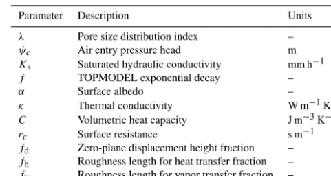
Table 1.The model parameters that need to be estimated.
Parameter Description Units
λ Pore size distribution index –
ψc Air entry pressure head m
Ks Saturated hydraulic conductivity mm h−1
f TOPMODEL exponential decay –
α Surface albedo –
κ Thermal conductivity W m−1K−1
C Volumetric heat capacity J m−3K−1
rc Surface resistance s m−1
fd Zero-plane displacement height fraction –
fh Roughness length for heat transfer fraction –
fv Roughness length for vapor transfer fraction –
More specifically, time-domain reflectometry (TDR)-based soil moisture observations and Bowen ratio-energy bal-ance (BREB)-based observations of the energy balbal-ance com-ponents in a large winter wheat field were available from 20 April to 5 July 2006, with the Bowen ratio data containing a number of gaps. The soil moisture was measured at a depth of 5, 9, 15, and 25 cm. Meteorologic data from the weather station at Görmin were available as well and can be used as model forcing from 2005 onwards. All observations were converted to an hourly time step by averaging the 10 min ob-servations. For this study, all model simulations were per-formed from 1 April 2006 to 5 July 2006, with an hourly time step, unless differently stated. A detailed description of this data set is given in Pauwels et al. (2008).
3 Model description
For the purpose of this study, the water and energy balance model developed in Scheerlinck et al. (2009) and applied in Pauwels and De Lannoy (2011) was used. Only a short de-scription will be provided in this section, and for a full model description we refer to Scheerlinck et al. (2009).
The model couples three physical equations. The move-ment of soil water in the unsaturated zone is mod-eled using a numerical solution of the Richards equation (Richards, 1931), which results in the profile of the pressure head (ψ; m). This equation requires the evapotranspiration as a boundary condition, which is calculated through an iter-ation of the surface energy balance, resulting in the surface skin temperature (Shuttleworth, 1992). This skin temperature is then used as a boundary condition for a numerical solution to the heat conduction equation, which results in the soil tem-perature profile (T; K).
obtained excellent results for the test site with this model. For this reason, the model is deemed sufficiently realistic.
The model is applied with four different uniform vertical spatial resolutions, namely, 0.01, 0.025, 0.05, and 0.1 m.
4 The parameter estimation algorithm: particle swarm optimization
4.1 General description
The parameter estimation algorithm used in this paper, par-ticle swarm optimization (PSO), is based on the collective behavior of individuals in decentralized, self-organizing sys-tems. These systems are created through a population of indi-viduals that interact locally with each other and with the com-munity. These interactions lead to global behavior, which can result in the achievement of certain objectives. Examples of such systems in nature are abundant: ant colonies, swarms of birds, and schools of fish (Kennedy and Eberhart, 1995). For a complete description of the algorithm we refer to Scheer-linck et al. (2009).
4.2 Application in this study
In order to estimate the model parameters, observations of the net radiation (Rn), latent heat flux (LE), sensible heat flux (H), ground heat flux (G), and soil moisture at 5 (θ1), 9 (θ2), 15 (θ3), and 25 cm (θ4) are used. The energy balance variables are in W m−2, and the soil moisture values are di-mensionless. A global objective function is calculated: OF=RMSERn
σRn
+RMSELE
σLE +
RMSEH σH +
RMSEG σG
+RMSEθ1 σθ1
+RMSEθ2 σθ2
+RMSEθ3 σθ3
+RMSEθ4 σθ4
. (1) The RMSE (root mean square error) values for each variable are calculated as
RMSEx= v u u t
1 Nx
Nx
X
i=1
(xo(i)−xs(i))2, (2)
wherexo andxs are the observed and simulated values, re-spectively, and σx is the standard deviation of the variable.
The global objective function is then minimized through the application of PSO; 36 iterations are performed, ensuring convergence of the algorithm, and the method is repeated 24 times. In order to ensure an analysis of the most opti-mal parameter values, the parameter sets corresponding to the eight lowest objective function values are retained for fur-ther analysis. More specifically, the average parameter and objective function values over these eight repetitions are ex-amined.
5 Model calibration using the numerically calculated ground heat flux
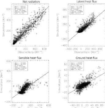
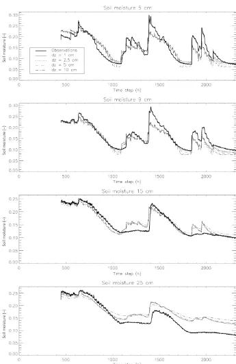
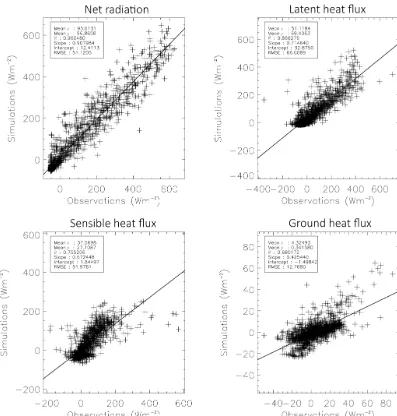
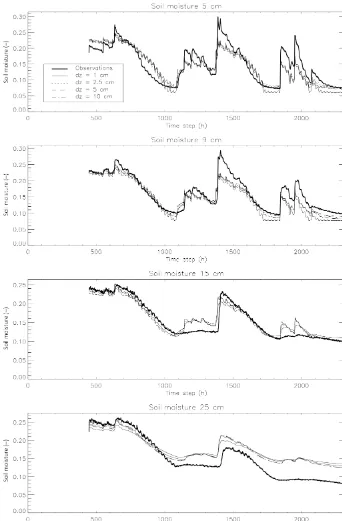
The model simulations resulting in the lowest objective func-tion values for the different spatial resolufunc-tions will be an-alyzed in this section. Figure 1 shows the comparison be-tween the modeled energy balance components and the ob-servations, for the spatial resolution of 0.01 m. Table 2 shows the statistics of the linear regressions between the observed and simulated energy balance components for the four spa-tial resolutions. Figure 2 shows the comparison between the modeled and the observed soil moisture values for the four spatial resolutions. From these figures and tables, it can be concluded that the model adequately simulated the water and energy balance processes, and that the results are very similar for the four different resolutions.
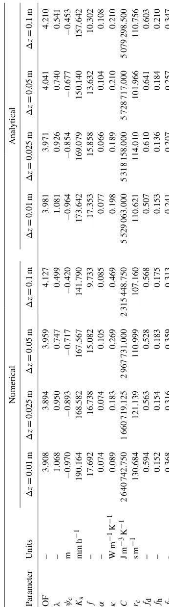
Table 3 shows the parameter values obtained from the model calibration with a spatial resolution of 0.01, 0.025, 0.05, and 0.1 m. In order to determine which parameters are significantly effected by the model spatial resolution, we ap-plied a t test to the slopes from the linear regressions be-tween the spatial resolution (x axis) and the parameter val-ues (y axis), at the 95 % confidence level. In other words, it is tested whether or not there is a significant linear trend between1z(the model resolution) and the parameter values. The objective function value has been found to change signif-icantly with the resolution, as well asλ,ψc,Ks,f, andκ. All
the other parameters are not significantly dependent on the spatial resolution. Of all the parameters affected by the reso-lution, the parameter that shows the largest variation in val-ues is the thermal conductivityκ, with the value at1z=0.1 being more than 4 times the value at1z=0.01 m. No other parameter shows such a dramatic variation.
Figure 1.Comparison between the modeled and the observed energy balance terms for the simulation with1z=0.01 m and a numerical solution of the heat conduction equation.
6 Analytical solution of the heat conduction equation 6.1 Derivation of the solution
In order to solve the issue related to the dependence on the grid resolution in the use of a numerical solution of the heat conduction equation, we propose the use of an analytical so-lution. First, the steady-state temperature profile for a con-stant temperature at the bottom (Tb,0) and top (Tu,0) of the profile is calculated. The depths of the top and bottom of the profile are denoted aszuandzb, respectively. This solution is then used as the initial condition for the same equation, now with different bottom (Tb,1) and top (Tu,1) temperatures as boundary conditions. It should be clarified that the timet starts at zero for this new solution. The temperature profile at time 1t is then calculated, and used as the initial condi-tion for the same equacondi-tion, again with different temperatures (Tb,2andTu,2) as boundary conditions, and time starting at zero. The solution at time1t is then again used as the ini-tial condition for the same equation with different boundary conditions (Tb,3andTu,3) and time starting at zero, and so on.
Using this recursive methodology, the temperature profile for theMth time step can be written as
T (z, t )= Tb,M−Tb,0 z−zu zb−zu
+ Tu,M−Tb,0 z−zb zu−zb
+Tb,0+2 Tb,M−Tb,M−1
∞
X
n=1 (−1)n
xn
sin
z−z
u zb−zu
xn
eynt+2 T
u,M−Tu,M−1
∞
X
n=1 (−1)n
xn
sin
z−zb zu−zbxn
eynt+2 M−1
X
m=1
Tb,m−Tb,m−1
∞
X
n=1 (−1)n
xn
sin
z−z
u zb−zu
xn
eyn[t+(M−m−1)1t]+2 M−1
X
m=1
Tu,m−Tu,m−1
∞
X
n=1 (−1)n
xn
sin
z−z
b zu−zb
xn
Table 2.Results of the linear regressions between the energy balance observations (xaxis) and the simulations (yaxis) for the simulations with a numerical solution of the heat conduction equation. Units are W m−2.
1z(m) x y Slope Intercept R RMSE
Rn
0.01 93.0131 100.600 0.915466 15.4496 0.960075 51.7281
0.025 98.3913 0.914448 13.3357 0.960305 51.3149
0.05 95.7262 0.885549 13.3586 0.959990 51.7374
0.1 98.1781 0.902939 14.1929 0.959981 51.5954
LE
0.01 51.1184 69.1110 0.743908 31.0836 0.876901 63.5272
0.025 68.2937 0.713683 31.8114 0.867113 65.5609
0.05 65.2262 0.703889 29.2445 0.875136 63.4643
0.1 68.7922 0.739403 30.9951 0.875059 63.8546
H
0.01 37.5698 26.7574 0.624850 3.28193 0.749120 51.9420
0.025 25.4533 0.680222 −0.102505 0.757655 52.2046
0.05 26.0201 0.627508 2.44475 0.749720 52.0724
0.1 25.0475 0.617920 1.83234 0.752516 51.9020
G
0.01 4.32493 4.74172 0.502091 2.57021 0.701958 11.7627
0.025 4.64757 0.505230 2.46248 0.709196 11.6390
0.05 4.48276 0.483105 2.39337 0.703112 11.7385
0.1 4.34807 0.471090 2.31064 0.702533 11.7558
where Tu,M andTb,M are the top and bottom temperatures (boundary conditions) for the Mth time step, with M >0, and
xn = nπ
yn = −
xn2κ C(zu−zb)2
. (4)
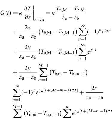
The surface ground heat flux then becomes
G(t )=κ ∂T ∂z
z=z
u
=κTu,M−Tb,M zu−zb
+ 2κ
zu−zb Tb,M−Tb,M−1
∞
X
n=1
(−1)neynt
+ 2κ
zu−zb Tu,M−Tu,M−1
∞
X
n=1 eynt
+ 2κ
zu−zb
M−1
X
m=1
Tb,m−Tb,m−1
∞
X
n=1
(−1)neyn[t+(M−m−1)1t]+ 2κ zu−zb
M−1
X
m=1
Tu,m−Tu,m−1
∞
X
n=1
eyn[t+(M−m−1)1t]. (5)
Appendix A describes the details of the derivation of this so-lution as well as a methodology to apply these equations in a computationally efficient manner.
It should be noted that with this analytical solution it is no longer necessary to calculate the soil temperature pro-file in order to calculate the ground heat flux. In the original model formulation, the heat conduction equation needed to be solved numerically, using the surface skin temperature as a boundary condition, so the temperature of the first soil layer could be calculated, and the ground heat flux could be com-puted. However, Eq. (5) shows that this first layer tempera-ture is no longer a variable in the calculation of the ground heat flux. More complex land surface models may contain parameters that depend on the soil temperature profile, and thus would require the application of Eq. (3). However, in this model, this is not required.
6.2 Comparison to the numerical solution
In a second application, a spatial resolution of 0.05 and a temporal resolution of 1 h (3600 s) are used. The air temper-ature values from the AgriSAR data set are used as boundary conditions at the top of the profile, and the bottom bound-ary conditions are assumed to linearly increase from 3 to 13◦ throughout the simulation.
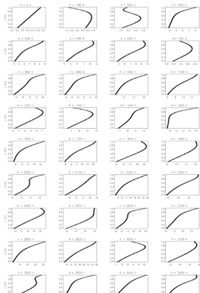
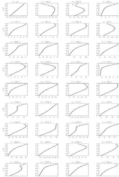
Figure 3 shows the comparison of the temperature profiles obtained from the numerical and analytical solutions, for the test case with the fine spatial and temporal resolutions. An excellent agreement between both methods can be seen. Fig-ure 4 shows the same comparison for the coarse resolutions. In many of these profiles, especially when sharp changes of temperature occur, a strong deviation of the numerical so-lution from the analytical soso-lution can be observed. Since these coarse resolutions correspond to values typically used in land surface models, this leads to the conclusion that care must be taken when interpreting ground heat flux simulations from these models. This is demonstrated in Fig. 5, in which the ground heat fluxes from both solutions are compared. For the fine resolutions, a very good agreement is obtained, but relatively strong differences between both methods are found when coarse spatial and temporal resolutions are used.
7 Model calibration using the analytically calculated ground heat flux
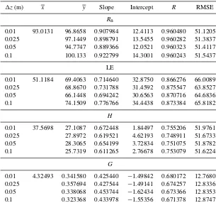
Figure 6 shows the comparison between the modeled energy balance terms and the observations, for the simulations with a spatial resolution of 0.01 m, and for the parameter set cor-responding to the lowest objective function value. A similar model performance as obtained with the numerical solution of the heat conduction equation is achieved. Table 4 shows the results of the linear regressions between the modeled en-ergy balance terms and the observations, again obtained us-ing the parameter values correspondus-ing to the lowest objec-tive function value, for the four different spatial resolutions. Comparing Tables 4 to 2 leads to the conclusion that the en-ergy balance terms are simulated practically identically when the model uses the numerical or the analytical solution of the heat conduction equation.
Figure 7 shows the comparison between the simulated soil moisture values and the observations for the same parameter sets. The comparison of Figs. 7 and 2 shows that the analyt-ical and numeranalyt-ical solutions of the heat conduction equation lead to very similar simulations of the soil water balance as well.
Table 3 shows the average parameter values from the eight retained PSO results. A slopettest for the linear regressions between the spatial resolutions (x axis) and the parameter values (y axis), at the 95 % confidence level, showed that the objective function value changes significantly with the resolution, as well asλ,ψc,Ks, andf. The only difference with the results obtained with the numerical solution of the heat conduction equation is thatκis no longer dependent on
[image:7.612.348.521.109.728.2]Table 4.Results of the linear regressions between the energy balance observations (xaxis) and the simulations (yaxis) for the simulations with an analytical solution of the heat conduction equation. Units are W m−2.
1z(m) x y Slope Intercept R RMSE
Rn
0.01 93.0131 96.8658 0.907984 12.4113 0.960480 51.1205
0.025 97.1449 0.898791 13.5455 0.960282 51.3837
0.05 94.7747 0.889366 12.0521 0.960323 51.4117
0.1 100.133 0.922799 14.3001 0.960243 51.5437
LE
0.01 51.1184 69.4063 0.714640 32.8750 0.866276 66.0089
0.025 68.8670 0.731788 31.4592 0.875547 63.8527
0.05 66.1448 0.694242 30.6563 0.870716 64.6836
0.1 74.1509 0.776766 34.4438 0.873384 65.8182
H
0.01 37.5698 27.1087 0.672448 1.84497 0.755206 51.9761
0.025 27.8972 0.619521 4.62193 0.748911 51.6733
0.05 28.3065 0.654199 3.72834 0.751075 51.8782
0.1 25.7319 0.611265 2.76678 0.753079 51.6224
G
0.01 4.32493 0.341580 0.425440 −1.49842 0.680172 12.7680
0.025 0.357694 0.427544 −1.49141 0.674257 12.8336
0.05 0.338068 0.453744 −1.62434 0.673366 12.8353
0.1 0.323368 0.433978 −1.55356 0.671378 12.8747
Figure 5.Comparison of the resulting ground heat fluxes from the fine and coarse spatial and temporal resolutions to the analytical solution.
the spatial resolution. This could be expected, because the expression for the ground heat flux is not dependent on the temperature of the first soil layer, and thus on the spatial res-olution. Furthermore, the value for the heat capacity (C) is now less variable than when the ground heat flux was calcu-lated numerically. More specifically, the standard deviation has been reduced from 557 943 to 278 984 J m−3K−1.
[image:10.612.90.246.408.654.2]Figure 6.Comparison between the modeled and the observed energy balance terms for the simulation where1z=0.01 m and an analytical solution of the heat conduction equation (Eq. A31).
The key conclusion from these simulations is that the over-all model performance is independent of the type of calcu-lation of the ground heat flux (analytically or numerically), but that the results of the model calibration are more robust (i.e., independent of the spatial resolution) if an analytical solution of the ground heat flux equation is used.
8 Conclusions
A water and energy balance model, using a numerical solution of the heat conduction equation, has been cali-brated against energy balance and soil moisture observations, for four different vertical spatial resolutions (0.01, 0.025, 0.05, and 0.1 m). It has been found that a number of param-eters are dependent on this resolution, with the soil thermal
Figure 7.Comparison between the modeled and the observed soil moisture values for the four different spatial resolutions, and an analytical solution of the heat conduction equation.
The results in this paper indicate that a similar model per-formance is obtained when the ground heat flux is calcu-lated analytically or numerically. However, the calibration is more robust, and the parameter values more physically inter-pretable, if the analytical solution is used. One must thus be careful when using numerical solutions of the heat
9 Data availability
Appendix A: Analytical solution A1 The governing equation
A solution of the heat conduction–convection equation is de-rived first, since this equation is analytically more straightfor-ward to solve than the heat conduction equation because of the easier inversion from the Laplace domain. Furthermore, this general solution can be used for purposes outside the scope of this paper. The limit case with zero convection is then calculated. The governing equation is
∂CT ∂t = ∂ ∂z κ∂T ∂z
−vC∂T
∂z, (A1) wheretis time (s),zis the depth positive upwards (m),T is the soil temperature (K), C is the volumetric heat capacity of the soil (J m−3K−1), κ is the soil thermal conductivity (W m−1K−1), andv is the water velocity (m s−1; positive upwards). We assume the parameters are uniform throughout the profile, so the equation becomes
C∂T ∂t =κ
∂2T ∂z2 −vC
∂T
∂z. (A2) A2 Steady-state solution
In order to obtain a realistic initial condition, we will calcu-late the steady-state solution. For example, the profile at the end of a very long, hot day. The equation becomes
κd 2T dz2 −vC
∂T
∂z =0, (A3) with the boundary conditions
T = Tb,0, z=zb
T = Tu,0, z=zu. (A4) The solution of this equation is
T =Tb,0+ Tb,0−Tu,0
evCκ z−evCκ zb evCκ zb−evCκ zu
. (A5) A3 Solution for first new boundary conditions
We will use a constant time steps1t. For the first new bound-ary conditions, we will use the steady-state profile as the ini-tial condition. The boundary conditions are
T = Tb,1, z=zb T = Tu,1, z=zu.
(A6) We will solve this equation through a Laplace transform. We will denote the transform of T (z,t )asF (z,y), withy the Laplace variable. The differential equation becomes
CyF−C Tb,0+ Tu,0−Tb,0 e vC
κ z−e vC
κ zb
evCκ zu−evCκ zb
!
=κd 2F dz2 −vC
dF
dz. (A7)
In the Laplace domain, the boundary conditions are
F = Tb,1
y , z=zb F = Tu,1
y , z=zu
. (A8)
The solution of this differential equation is
F = Tb,1−Tb,0
eb(z
−zb) y
sinh
q
b2+Cy
κ (z−zu)
sinh
q
b2+Cy
κ (zb−zu)
+ Tu,1−Tu,0e
b(z−zu) y
sinh
q
b2+Cy
κ (z−zb)
sinh
q
b2+Cy
κ (zu−zb)
+1
y Tu,0−Tb,0
e
vC
κ z−evCκ zb evCκ zu−evCκ zb
+Tb,0
y , (A9) wherebis defined as
b=Cv
2κ. (A10)
We will calculate the poles of this equation (the values fory for which the denominator is zero), and calculate the resid-uals of each pole. The analytical solution is then simply the sum of the residuals (Brutsaert, 1994). Following this theo-rem, writingF (y)asP (y)/T (y), we can write
Ri= lim y→yi
(y−yi)
P (y)eyt T (y)
. (A11)
If the pole cannot be factored out, this becomes Ri=
P (yi) eyit ∂T (y)
∂y
y=yi
. (A12)
Equation (A9) has poles fory equal to zero and for the hy-perbolic sine equal to zero. Fory equal to zero this simply becomes
T1(z)= Tb,1−Tb,0eb(z−zb)
sinh(b (z−zu)) sinh(b (zb−zu))
+ Tu,1−Tu,0eb(z−zu)
sinh(b (z−zb)) sinh(b (zu−zb))
+ Tu,0−Tb,0
evCκ z−evCκ zb evCκ zu−evCκ zb
+Tb,0. (A13)
For the hyperbolic sine, we define
r
b2+Cy
wherej is the complex variable (
√
−1). We can now write
sinh
r
b2+Cy
κ (zu−zb)
!
=jsin(x). (A15)
This is equal to zero forx=nπ, withn=0, 1, 2, etc. This means thatyis equal to
b2+Cyn
κ
(zu−zb)2= −xn2⇒yn
= − x
2
nκ
C(zu−zb)2
−κb
2
C , (A16)
wherexn=nπ. We can thus write the solution as
T2(z, t )= − Tb,1−Tb,0 2κ C(zu−zb)2e
b(z−zb)
∞
X
n=1 (−1)n xn
yn
sin
z−z
u zb−zuxn
eynt− T
u,1−Tu,0
2κ C(zu−zb)2e
b(z−zu)
∞
X
n=1
(−1)nxn yn
sin
z−zb zu−zbxn
eynt. (A17)
The analytical solution is then simply
T (z, t )=T1(z)+T2(z, t ). (A18) A4 Solution for second new inputs
We will calculate the temperature profile att =1t, and use this as the initial condition for the same equation. The bound-ary conditions are
T = Tb,2, z=zb T = Tu,2, z=zu.
(A19) In the Laplace domain, the differential equation becomes CyF−C Tb,1−Tb,0eb(z−zb) sinh(b (z−zu))
sinh(b (zb−zu))
−C Tu,1−Tu,0eb(z−zu) sinh(b (z−zb)) sinh(b (zu−zb))
−C Tu,0−Tb,0 e vC
κ z−e vC
κ zb
evCκ zu−evCκ zb
−CTb,0
+C Tb,1−Tb,0 2κ C(zu−zb)2
eb(z−zb)
∞
X
n=1
(−1)nxn yn
sin
z−z
u zb−zuxn
eyn1t
+C Tu,1−Tu,0 2κ C(zu−zb)2e
b(z−zu)
∞
X
n=1
(−1)nxn yn
sin
z−z
b zu−zb
xn
eyn1t
=κd 2F dz2 −vC
dF
dz. (A20)
The boundary conditions are, in the Laplace domain
F = Tb,2
y , z=zb F = Tu,2
y , z=zu
. (A21)
F can then be written as
F = Tb,2−Tb,1 eb(z−zb)
y
sinh
q
b2+Cy
κ (z−zu)
sinh
q
b2+Cy
κ (zb−zu)
+ Tu,2−Tu,1
e b(z−zu)
y
sinh
q
b2+Cy
κ (z−zb)
sinh
q
b2+Cy
κ (zu−zb)
+1
y Tb,1−Tb,0
eb(z−zb) sinh(b (z−zu)) sinh(b (zb−zu))
+1
y Tu,1−Tu,0
eb(z−zu) sinh(b (z−zb)) sinh(b (zu−zb))
+1
y Tu,0−Tb,0
e
vC κ z−e
vC κ zb
evCκ zu−evCκ zb
+Tb,0
y
− Tb,1−Tb,0 2κ C(zu−zb)2e
b(z−zb)
∞
X
n=1 (−1)n xn
yn(y−yn)
sin
z−zu zb−zuxn
eyn1t
− Tu,1−Tu,0 2κ C(zu−zb)2e
b(z−zu)
∞
X
n=1 (−1)n xn
yn(y−yn)
sin
z−zb
zu−zbxn
eyn1t. (A22)
Through calculating the poles and the residuals, the inverse transform is
T (z, t )= Tb,2−Tb,0eb(z−zb) sinh(b (z−zu)) sinh(b (zb−zu))
+ Tu,2−Tu,0eb(z−zu) sinh(b (z−zb)) sinh(b (zu−zb))
+ Tu,0−Tb,0 e vC
κ z−e vC
κ zb
evCκ zu−evCκ zb
+Tb,0
− Tb,2−Tb,1 2κ C(zu−zb)2e
b(z−zb)
∞
X
n=1 (−1)n xn
yn
sin
z−zu zb−zuxn
eynt
− Tu,2−Tu,1 2κ C(zu−zb)2e
b(z−zu)
∞
X
xn
yn
sin
z−zb
zu−zb xn
eynt
− Tb,1−Tb,0 2κ C(zu−zb)2
eb(z−zb)
∞
X
n=1 (−1)n xn
yn
sin
z−z
u zb−zu
xn
eyn(t+1t )
− Tu,1−Tu,0 2κ C(zu−zb)2
eb(z−zu)
∞
X
n=1 (−1)n xn
yn
sin
z−z
b zu−zb
xn
eyn(t+1t ). (A23) A5 Solution forMsequential boundary conditions Through again calculating the temperature profile at timet equal to 1t, using this as input for the governing equation with new boundary conditions, and applying this methodol-ogy recursively, the temperature profile for boundary condi-tionsTu,MandTb,Mas
T (z, t )= Tb,M−Tb,0eb(z−zb) sinh(b (z−zu)) sinh(b (zb−zu))
+ Tu,M−Tu,0eb(z−zu) sinh(b (z−zb)) sinh(b (zu−zb))
+ Tu,0−Tb,0
e
vC
κ z−evCκ zb evCκ zu−evCκ zb
+Tb,0
− Tb,M−Tb,M−1 2κ C(zu−zb)2e
b(z−zb)
∞
X
n=1 (−1)n xn
yn
sin
z−zu
zb−zuxn
eynt
− Tu,M−Tu,M−1 2κ C(zu−zb)2e
b(z−zu)
∞
X
n=1 (−1)n xn
yn
sin
z−zb
zu−zb xn
eynt
− 2κ
C(zu−zb)2 eb(z−zb)
M−1
X
m=1
Tb,m−Tb,m−1
∞
X
n=1
(−1)nxn yn
sin
z−z
u zb−zu
xn
eyn[t+(M−m−1)1t]
− 2κ
C(zu−zb)2 eb(z−zu)
M−1
X
m=1
Tu,m−Tu,m−1
∞
X
n=1
(−1)nxn ynsin
z−zb
zu−zb
xn
eyn[t+(M−m−1)1t]. (A24)
Calculating the first derivative with respect to zat zu and multiplying by the thermal conductivity leads to the ground heat flux:
G(t )=κ Tu,M−Tb,M−Tu,0+Tb,0
beb(zu−zb) sinh(b (zu−zb))
+vC Tu,0−Tb,0 e vC
κ zu
evCκ zu−evCκ zb 2κ2
C(zu−zb)3
eb(zu−zb)
∞
X
n=1
(−1)n− Tb,M−Tb,M−1 xn2
yn
eynt− Tu,M−Tu,M
−1 2κ2 C(zu−zb)3
∞
X
n=1 xn2 yn
eynt
− 2κ
2
C(zu−zb)3
eb(zu−zb) M−1
X
m=1
Tb,m−Tb,m−1
∞
X
n=1 (−1)n xn2
yn
eyn[t+(M−m−1)1t]− 2κ 2
C(zu−zb)3
M−1
X
m=1 Tu,m−Tu,m−1
∞
X
n=1 xn2 yn
eyn[t+(M−m−1)1t]. (A25) A6 Computationally efficient formulation
For the temperature profile, we define two variablesτt(z,n) andτb(z,n)for each value ofz, which are initially zero. In general, we write the solution for temperature inputMas T (z, t )= Tb,M−Tb,0eb(z−zb)
sinh(b (z−zu)) sinh(b (zb−zu))
+ Tu,M−Tu,0
eb(z−zu) sinh(b (z−zb)) sinh(b (zu−zb))
+ Tu,0−Tb,0
evCκ z−evCκ zb evCκ zu−evCκ zb
+Tb,0
− Tb,M−Tb,M−1
2κ
C(zu−zb)2 eb(z−zb)
∞
X
n=1 (−1)n xn
yn
sin
z−z
u zb−zu
xn
eynt− Tu,M−Tu,M
−1 2κ
C(zu−zb)2 eb(z−zu)
∞
X
n=1
(−1)nxn yn
sin
z−zb zu−zbxn
eynt− 2κ C(zu−zb)2
eb(z−zb)
∞
X
n=1 τb,neynt
− 2κ
C(zu−zb)2e
b(z−zu)
∞
X
n=1
τt,neynt. (A26)
At the end of the time step we update the variables:
τb(z, n)→τb(z, n)eyn1t+Tb,M−Tb,M−1(−1)n
xn
yn
sin
z−zu
zb−zu
xn
eyn1t
τt(z, n)→τt(z, n)eyn1t+Tu,M−Tu,M−1(−1)n
xn
yn
sin
z−zb
zu−zb
xn
eyn1t . (A27)
For the ground heat flux, we define two variablesψt(n)and ψb(n), again initially zero. We then write the ground heat flux as
G(t )=κ Tu,M−Tb,M−Tu,0+Tb,0 be
b(zu−zb) sinh(b (zu−zb))
+vC Tu,0−Tb,0
e
vC κ zu
− Tb,M−Tb,M−1
2κ
2
C(zu−zb)3
eb(zu−zb)
∞
X
n=1 (−1)n xn2
yn
eynt− T
u,M−Tu,M−1
2κ2 C(zu−zb)3
∞
X
n=1 xn2 yn
eynt
− 2κ
2
C(zu−zb)3e
b(zu−zb)
∞
X
n=1
ψb(n)eynt
− 2κ
2
C(zu−zb)3
∞
X
n=1
ψt(n)eynt. (A28)
At the end of each time step we then update
ψb(n)→ψb(n)eyn1t+ Tb,M−Tb,M−1
(−1)nx
2
n
yn
eyn1t
ψt(n)→ψt(n)eyn1t+ Tu,M−Tu,M−1 x
2
n
yn
eyn1t
. (A29)
A7 Limit case for zero convection
In this case b becomes zero. We can rewrite Eq. (A24) as (using de l’Hôpitals’s rule)
T (z, t )= Tb,M−Tb,0 z−zu
zb−zu+ Tu,M−Tb,0
z−zb
zu−zb
+Tb,0+2 Tb,M−Tb,M−1
∞
X
n=1
(−1)n xn sin
z−zu
zb−zu
xn
+eynt2 Tu,M−Tu,M
−1
∞
X
n=1 (−1)n
xn
sin
z−z
b zu−zb
xn
eynt+2 M−1
X
m=1
Tb,m−Tb,m−1
∞
X
n=1 (−1)n
xn
sin
z−z
u zb−zu
xn
eyn[t+(M−m)1t]+2 M−1
X
m=1 Tu,m−Tu,m−1
∞
X
n=1 (−1)n
xn
sin
z−z
b zu−zbxn
eyn[t+(M−m)1t]. (A30)
The ground heat flux then becomes
G(t )=κTu,M−Tb,M zu−zb
+ 2κ
zu−zb
Tb,M−Tb,M−1
∞
X
n=1 (−1)n
eynt+ 2κ zu−zb
Tu,M−Tu,M−1
∞
X
n=1
eynt+ 2κ zu−zb
M−1
X
m=1
Tb,m−Tb,m−1
∞
X
n=1
(−1)neyn[t+(M−m)1t]
+ 2κ
zu−zb M−1
X
m=1
Tu,m−Tu,m−1
∞
X
n=1
eyn[t+(M−m)1t]. (A31)
Author contributions. Edoardo Daly and Valentijn R. N. Pauwels developed the idea to use an analytical solution to model the ground heat flux in land surface models, instead of numerical so-lutions. Valentijn R. N. Pauwels solved the equation, prepared the manuscript, and performed the model simulations. The results were extensively discussed and analyzed by both authors.
Acknowledgements. Valentijn R. N. Pauwels is funded through Australian Research Council Future Fellowship grant num-ber FT130100545.
Edited by: P. Gentine
Reviewed by: J. Wang and two anonymous referees
References
Bennett, W. B., Wang, J. F., and Bras, R. L.: Estimation of global ground heat flux, J. Hydrometeorol., 9, 744–759, 2008. Brutsaert, W.: The unit response of groundwater outflow from a
hill-slope, Water Resour. Res., 30, 2759–2763, 1994.
Carslaw, H. S. and Jaeger, J. C.: Conduction of heat in solids, Clarendon Press, Oxford, 1959.
Cichota, R., Elias, E. A., and van Lier, Q. D.: Testing a finite-difference model for soil heat transfer by comparing numerical and analytical solutions, Environ. Model. Softw., 19, 495–506, 2004.
Gao, Z. Q., Fan, X. G., and Bian, L. G.: An analytical so-lution to one-dimensional thermal conduction-convection in soil, Soil Sci., 168, 99–107, doi:10.1097/00010694-200302000-00004, 2003.
Gentine, P., Polcher, J., and Entekhabi, D.: Harmonic propagation of variability in surface energy balance within a coupled soil– vegetation–atmosphere system, Water Resour. Res., 48, W05525, doi:10.1029/2010WR009268, 2011.
Gentine, P., Entekhabi, D., and Heusinkveld, B.: Systematic errors in ground heat flux estimation and their correction, Water Resour. Res., 48, W09541, doi:10.1029/2010WR010203, 2012. Hu, G., Zhao, L., Wu, X., Li, R., Wu, T., Xie, C., Qiao, Y.,
Shi, J., Li, W., and Cheng, G.: New Fourier-series-based an-alytical solution to the conduction-convection equation to cal-culate soil temperature, determine soil thermal properties, or estimate water flux, Int. J. Heat Mass Transf., 95, 815–823, doi:10.1016/j.ijheatmasstransfer.2015.11.078, 2016.
Kennedy, J. and Eberhart, R. C.: Particle Swarm Optimization, in: Proc. IEEE In. Conf. Neur. Netw., Piscataway, NJ, 1942–1948, 1995.
Liebethal, C. and Foken, T.: Evaluation of six parameterization ap-proaches for the ground heat flux, Theor. Appl. Climatol., 88, 43–56, doi:10.1007/s00704-005-0234-0, 2007.
Lunati, I., Ciocca, F., and Parlange, M. B.: On the use of spatially discrete data to compute energy and mass balance, Water Resour. Res., 48, W05542, doi:10.1029/2012WR012061, 2012. Nunez, C. M., Varas, E. A., and Meza, F. J.: Modelling soil heat flux,
Theor. Appl. Climatol., 100, 251–260, doi:10.1007/s00704-009-0185-y, 2010.
Orth, R. and Seneviratne, S.: Using soil moisture forecasts for sub-seasonal summer temperature predictions in Europe, Clim. Dy-nam., 43, 3403–3418, doi:10.1007/s00382-014-2112-x, 2014. Pauwels, V. R. N. and De Lannoy, G. J. M.: Multivariate
calibra-tion of a water and energy balance model in the spectral domain, Water Resour. Res., 47, W07523, doi:10.1029/2010WR010292, 2011.
Pauwels, V. R. N., Timmermans, W., and Loew, A.: Comparison of the estimated water and energy budgets of a large winter wheat field during AgriSAR 2006 by multiple sensors and models, J. Hydrol., 349, 425–440, 2008.
Richards, L.: Capillary conduction of liquids through porous media, Physics, 1, 318–333, 1931.
Russell, E. S., Liu, H. P., Gao, Z. M., Finn, D., and Lamb, B.: Impacts of soil heat flux calculation methods on the surface energy balance closure, Agr. Forest Meteorl., 214, 189–200, doi:10.1016/j.agrformet.2015.08.255, 2015.
Scheerlinck, K., Pauwels, V. R. N., Vernieuwe, H., and De Baets, B.: Calibration of a water and energy balance model: Recursive Pa-rameter Estimation versus Particle Swarm Optimization, Water Resour. Res., 10, W10422, doi:10.1029/2009WR008051, 2009. Shao, M., Horton, R., and Jaynes, D. B.: Analytical Solution for
One-Dimensional Heat Conduction-Convection Equation, Soil Sci. Am. J., 62, 123–128, 1998.
Shuttleworth, W. J.: Evaporation, McGraw-Hill, New York, NY, 4.1–4.53, 1992.
Venegas, P., Grandon, A., Jara, J., and Paredes, J.: Hourly estima-tion of soil heat flux density at the soil surface with three mod-els and two field methods, Theor. Appl. Climatol., 112, 45–59, doi:10.1007/s00704-012-0705-z, 2013.
Wang, L., Gao, Z., Horton, R., Lenschow, D. H., Meng, K., and Jaynes, D. B.: An Analytical Solution to the One-Dimensional Heat Conduction-Convection Equation in Soil, Soil Sci. Am. J., 76, 1978–1986, doi:10.2136/sssaj2012.0023N, 2012.