How streamflow has changed across Australia since the 1950s: evidence from the network of hydrologic reference stations

www.hydrol-earth-syst-sci.net/20/3947/2016/ doi:10.5194/hess-20-3947-2016

© Author(s) 2016. CC Attribution 3.0 License.

How streamflow has changed across Australia since the 1950s:

evidence from the network of hydrologic reference stations

Xiaoyong Sophie Zhang1, Gnanathikkam E. Amirthanathan1, Mohammed A. Bari2, Richard M. Laugesen3, Daehyok Shin1, David M. Kent1, Andrew M. MacDonald1, Margot E. Turner1, and Narendra K. Tuteja3 1_{Environment and Research Division, Bureau of Meteorology, Melbourne, Australia}

2_{Bureau of Meteorology, Perth, Australia} 3_{Bureau of Meteorology, Canberra, Australia}

Correspondence to:Xiaoyong Sophie Zhang ([email protected])

Received: 3 November 2015 – Published in Hydrol. Earth Syst. Sci. Discuss.: 18 January 2016 Revised: 10 August 2016 – Accepted: 27 August 2016 – Published: 26 September 2016

Abstract. Streamflow variability and trends in Australia were investigated for 222 high-quality stream gauging sta-tions having 30 years or more continuous unregulated streamflow records. Trend analysis identified seasonal, inter-annual and decadal variability, long-term monotonic trends and step changes in streamflow. Trends were determined for annual total flow, baseflow, seasonal flows, daily maxi-mum flow and three quantiles of daily flow. A distinct pat-tern of spatial and temporal variation in streamflow was evident across different hydroclimatic regions in Australia. Most of the stations in southeastern Australia spread across New South Wales and Victoria showed a significant decreas-ing trend in annual streamflow, while increasdecreas-ing trends were retained within the northern part of the continent. No strong evidence of significant trend was observed for stations in the central region of Australia and northern Queensland. The findings from step change analysis demonstrated evidence of changes in hydrologic responses consistent with observed changes in climate over the past decades. For example, in the Murray–Darling Basin, 51 out of 75 stations were iden-tified with step changes of significant reduction in annual streamflow during the middle to late 1990s, when relatively dry years were recorded across the area. Overall, the hydro-logic reference stations (HRSs) serve as critically important gauges for streamflow monitoring and changes in long-term water availability inferred from observed datasets. A wealth of freely downloadable hydrologic data is provided at the HRS web portal including annual, seasonal, monthly and daily streamflow data, as well as trend analysis products and relevant site information.

1 Introduction

Assessing changes and trends in streamflow observations can provide vital information for sustainable water resource management. The influence of diverse environmental fac-tors and anthropogenic changes on hydrological behaviour makes the investigation into streamflow changes a challeng-ing task. Trend detection is further complicated from intra-annual, inter-intra-annual, decadal and inter-decadal variability in streamflow as well as from various influencing factors that can hardly been analysed separately (WWAP, 2012; Hen-nessy et al., 2007).

range of research on streamflow trends has been published in the USA (Kumar et al., 2009; Novotny and Stefan, 2007; Mc-Cabe and Wolock, 2002) and Canada (Bawden et al., 2014; Monk et al., 2011; Burn and Hag Elnur, 2002).

Few studies have been published for Australia to date partly due to limited information on data records, research and documentation that could cover all flow regimes. Rivers in some regions have received close attention only recently. Australia is the driest inhabited continent with an average an-nual precipitation of 450 mm and the lowest river flow com-pared with other continents (Poff et al., 2006). Water is rel-atively scarce and is therefore a valuable resource across the country. Australian streams are characterized by low runoff, high inter-annual flow variability and large magnitudes of variations between the maximum and minimum flows (Puck-ridge et al., 1998; Finlayson and McMahon, 1988). The wide variety of unique topographic features combined with vari-able climates and frequency in weather extremes result in di-verse flow regimes. The recent rise in average temperature and the risk of future climate variability (BOM, 2016; IPCC, 2014; Cleugh et al., 2011) have added new dimensions to the challenges already facing communities. Climate variability and its impact on the hydrologic cycle have necessitated a growing need in Australia to seek evidence of any emerging trends in river flows.

Chiew and McMahon (1993) examined the annual stream-flow series of 30 unregulated Australian rivers to detect trends or changes in the means. They found that identified changes in the tested dataset were directly related to the inter-annual variability rather than changes in climate. The analy-sis of trends in Australian flood data by Ishak et al. (2010) indicated that about 30 % of the selected 491 stations show trends in annual maximum flood series data, with a down-ward trend in the southern part of Australia and an updown-ward trend in the northern part. Several other studies investigated trends of selected streamflow statistics in a particular region, e.g. southwest Australia (Petrone et al., 2010; Durrant and Byleveld, 2009), southeast Australia or Victoria (Tran and Ng, 2009; Stewardson and Chiew, 2009). All these studies addressed the trend analysis of Australian rivers with a lim-ited spatial or temporal coverage of flow data. A gap in the research remains mainly due to constraints in the access to a dataset of catchments that can be large enough to represent the diversity of flow regimes across Australia. Such a dataset would enable a comprehensive and systematic appraisal of changes and trends in observed river flow records.

The Australian national network of hydrologic reference stations (HRSs) was developed by the Bureau of Meteorol-ogy to address this major gap and to provide comprehensive analysis of long-term trends in water availability across the country (Zhang et al., 2014; Turner et al., 2012). The HRS website is a one-stop portal to access high-quality streamflow information for 222 well-maintained river gauges in near-natural catchments. An intention is that the stations will serve as critically important gauges that record and detect changes

in hydrologic responses to long-term climate variability and other factors.

This paper presents a statistical analysis to detect changes or emerging trends across a range of flow indicators, based on the daily flow data of 222 sites from the HRS network. The objective of this study is to provide a nationwide assessment of the long-term trends in observed streamflow data. Eval-uation of past streamflow records and documenting recent trends will be of benefit in anticipating potential changes in water availability and flood risks. It is hoped that the find-ings from trend analysis presented in this paper will inform decision makers on long-term water availability across dif-ferent hydroclimatic regions and be used for water security planning within a risk assessment framework.

2 Site selection, data and methods

2.1 Hydrologic reference stations and data

The 222 HRSs were selected from a preliminary list of potential streamflow stations across Australia according to the HRS selection guideline (SKM, 2010). These guidelines specified four criteria for identifying the high-quality ref-erence stations, namely unregulated catchments with mini-mal land use change, a long period of record (greater than 30 years) of high-quality streamflow observations, spatial representativeness of all hydroclimate regions and the impor-tance of site as assessed by stakeholders. Catchments with extensive basin water use or groundwater pumping were fil-tered and not included in HRS catchments, based on the local knowledge of the basin, stakeholder consultation and land use change analysis. The station selection guidelines were then applied in four phases to finalise the station list (http:// www.bom.gov.au/water/hrs/guidelines.shtml). The HRS net-work will be reviewed and updated every 2 years to ensure that the high quality of the streamflow reference stations is maintained.

Table 1.Metadata of the drainage divisions and HRSs.

Division Drainage division Mean Mean Number Water Smallest Largest

map names annual elevation of HRS year catchment catchment

code rainfall (m) stations start area area

(mm) month (km2) (km2)

(1976–2005)∗

I Northeast Coast 764 173 42 October 6.6 7486.7

II Southeast Coast 599 323 44 March 4.5 4660.0

III Tasmanian 1519 199 12 February 18.3 775.3

IV Murray–Darling 479 260 75 March 26.3 35238.9

V South Australia Gulf 344 269 5 February 5.3 187.4

VI Southwest Coast 329 365 13 March 14.1 1786.0

VII Indian Ocean 369 162 0 (no data) (no data) (no data)

VIII Timor Sea 520 339 13 September 65.4 47651.5

IX Gulf of Carpentaria 674 293 13 October 170.0 43476.2

X Lake Eyre 429 312 5 October 434.9 232846.3

XI North Western Plateau 456 359 0 (no data) (no data) (no data)

XII South Western Plateau 321 297 0 (no data) (no data) (no data)

∗_{Calculation was based on rainfall data from BOM climate website http://www.bom.gov.au/.}

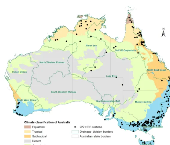
Figure 1.Location of the 222 high-quality streamflow reference stations, the climatic regions and Australia drainage divisions (Geofabric

surface hydrology catchments, Geofabric V2.1; BOM, 2015).

of stations along the coast and sparsely distributed stations across inland areas. One-third of the HRS sites are in tem-perate climate zone, and the majority of the rest are either in tropical or subtropical regions; only a few are located in other climate zones. The distribution of HRSs across multi-ple hydroclimatic regions provides data for a comprehensive investigation of long-term streamflow variability across Aus-tralia.

constitute the first such statement on long-term water avail-ability across Australia.

The earliest record included in the dataset is from 1950. Data prior to this have been excluded due to the common ex-istence of large gaps in the pre-1950 period. All stations in-cluded in the HRS had a target of 5 % or less missing data to meet the completeness criteria for high-quality stream-flow records. A few stations were included with more than 5 % missing data where they excelled in other criteria such as stakeholder importance or spatial coverage. The peri-ods of data gaps were filled using a lumped rainfall–runoff model GR4J (Perrin et al., 2003). The gap filling was found to perform well at most sites. The mean Nash–Sutcliffe co-efficient of the gap-filled time series, when compared to the available original time series data, was 0.72 with stan-dard deviation of 0.12. The model was calibrated and forced with catchment average rainfall and potential evapotranspira-tion from the Australian Water Availability Project (AWAP) (Raupach et al., 2009).

The study examined all sites using the full length of ob-servations after 1950. Prior to 1950, the gauge network is generally too sparse for reliable analysis, and analysis peri-ods starting after the mid-1970s are considered too short to calculate meaningful trend values. Although, the data length of every station was not exactly the same over the continent, but for the stations within the same region, the data lengths were in more consistent time periods. Data for most of sta-tions (86 %) have very similar time periods. These allow for comparisons on a fairly consistent basis.

The gap-filled daily flow data were aggregated into annual series based on a water year calculation. The start month of the water year was defined as the month with the low-est monthly flow across the available data period. The start month of water year for each region was recorded in Table 1. The data used in this study were up to the end of 2014, so the last water year cycle ended in 2014. In order to ensure the statistical validity of the trend analysis, all stations had minimum 30 years of record, with mean time series length of 48 years and median time series length of 46.6 years. The longest record length was 64 years. A total of 25 % of the stations have 50 or more years of record and 86 % stations longer than 40 years of data. Catchment sizes ranged from 4.5 to 232 846 km2 with a median size of 328.6 km2. The majority (80 %) of the stations had an upstream drainage area less than 800 km2, and only three stations had a drainage area larger than 50 000 km2.

The primary water data have been collected across Aus-tralia by many organisations, utilities and regulators in dif-ferent states and territories, often to meet the requirements of their own documented procedures and sometimes with ref-erence to Australian or international standards or guidelines. The bureau’s role as the national water information provider has been working collaboratively with the water industry to develop and promote water information standards and guide-lines to collate, interpret and access nationally consistent

data. All data included in the HRS database are compiled, quality checked by the bureau and therefore are consistent nationally and over the time. The bureau has developed a set of standard data quality code and references guides on how it relates to different agencies quality code. The data and the long-term series gathered in this study are the best compiled and quality-assured data for HRS catchments. The analysis and trends derived from the HRS datasets constitute the first statement on long-term water availability across Australia.

2.2 Streamflow variables for trend analysis

Long-term climate variability can be reflected through trends in streamflow variables. To understand the importance of the components of the hydrologic regimes and their poten-tial link to long-term climate variability, 10 streamflow ables were chosen for statistical and trend analysis. Two vari-ables related to fluctuation of annual flows were annual total flow (QT) and annual baseflow (QBF). Baseflow was sepa-rated from daily total streamflow using a digital filter based on theory developed by Lyne and Hollick (1979) and applied by Nathan and McMahon (1990).

Daily streamflow data were analysed to form a group of indicators of daily flow trends. They were daily maximum flow (QMax), the 90th percentile (non-exceedance probabil-ity) daily flow (Q90), the 50th percentile daily flow (Q50) and the 10th percentile daily flow of each year (Q10). The median daily flowQ50was used in the study instead of daily mean flow because the flow distribution is skewed and outliers are present.

Four seasonal flow indicators were analysed to examine the seasonal trend patterns. These variables included sum-mer flowQDJF(December to February), autumn flowQMAM (March to May), winter flow QJJA (June to August) and spring flowQSON(September to November). The trend anal-ysis was applied to the 10 hydrologic indicators of stream-flow data at each HRS station.

2.3 Trend and data statistical analysis

study attempted to examine patterns in raw historical stream-flow records, no further adjustments were made to account for the non-random structure of data.

The non-parametric MK trend test was used to detect the direction and significance of the monotonic trend, and the trend line by the non-parametric Sen slope (Sen, 1968; Theil, 1950) was used to approximately represent the magnitude of the trend. The trend magnitude was standardised using the ratio of Sen slope coefficient to average annual flow in order to make the change comparable across stations for reporting purposes.

All data were subject to step change analysis to detect any abrupt changes during the record period. The distribution-free CUSUM test (Chiew and Siriwardena, 2005) was ap-plied to identify the year of change in streamflow series. The significant difference between the median of the streamflow series before and after the year of change was tested by rank– sum method (Zhang et al., 2010; Miller and Piechota, 2008; Chiew and Siriwardena, 2005). More information and equa-tions of the statistical tests used in this study can be found in Appendix A.

In addition to the trend analysis for the 10 flow indicators, other statistical data analyses were included in the HRS web portal to gain a broad understanding of hydrologic regimes. Aggregated monthly and seasonal flow data were investi-gated for changes in flow patterns in different basins or re-gions. Daily event frequency analyses were used to examine the variations in daily streamflow magnitude, and daily flow duration curves were presented to examine changes in daily flow among decades.

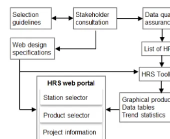
3 Development of the HRS web portal

A web portal has been developed to house the network of HRSs and provide access to streamflow data, results of anal-ysis and associated site information. Figure 2 summarises the development process of the HRS network and web-site. Through a data quality assurance process following the guidelines and stakeholder consultations, the final list of 222 streamflow gauging stations was established. A suite of software tools, “the HRS toolkit” was developed to under-take data aggregation, analysis, trend testing, visualisation and manipulation. The toolkit is capable of automatically converting the flow variables to monthly, seasonal and an-nual totals, and quantifying the step and/or linear changes in the selected streamflow variables. The toolkit also generated and processed graphical products, data, statistical summary tables and statistical metadata included in the web portal.

A snapshot of the HRS web portal is shown in Fig. 3. The main page was designed with three parts. A series of links on the top provide the project information. Below this is the station selector, which facilitates searching for the site of in-terest by location. The third part is the product selector con-taining the core information sections of the website. Several

Figure 2.Framework of developing HRSs.

tabs are offered for users to explore the web portal dependent on their needs and the level of information they require. The daily streamflow data, graphical products, statistics and trend analysis results are available for users to view and down-load. Information provided on the HRS web portal will assist in detecting long-term streamflow variability and changes at the 222 sites and therefore supports water planning and deci-sion making. More information can be found at the website http://www.bom.gov.au/water/hrs.

This web portal provides public access to high-quality data and information. It has more than 15 000 graphic products for display. It is carefully designed for the public to have synthe-sised and easily understandable information on water avail-ability trends across Australia. In order to ensure currency of this web site, streamflow data are updated and reviewed every 2 years.

4 Results

The study to detect long-term streamflow trends was per-formed on the 222 gauging stations included in the HRS net-work. This section presents an overview bar plot of the MK test results for the selected 10 hydrologic variables. Maps showing trend detection results and step change analysis for the annual total flow are presented as well as a table list-ing the stations with significant trends in annual total flow at 1 % significance level (p <0.01). In addition, result statistics of trends and step changes were summarised for different re-gions. Finally, variations in trend among daily flow indicators and seasonal flows were examined.

4.1 Overview

Figure 3.Snapshot of the HRS web portal.

Figure 4.Stacked bar plot summarising the MK trend test results for the 222 HRS stations, with data labels showing the number of

sta-tions in each category (QT: annual total flow,QBF: annual baseflow,Qmax: daily maximum flow,Q90: 90th percentile daily flow,Q50: 50th percentile daily flow,Q₁₀: 10th percentile daily flow,QDJF: summer flow,QMAM: autumn flow,QJJA: winter flow,QSON: spring flow).

Patterns of trends were noted in the different flow regimes. Moving through the flow variables from low (Q10), me-dian (Q50), high (Q90) and to maximum (QMax), an increas-ing number of stations were found with no trends, combined with decreasing number for non-random series. The overall number of stations with statistically significant trends was around the same across the median, high and maximum vari-ables but much lower for the low flow variable. In the trends

non-Figure 5.Spatial variation in trend results of annual total flow (QT); trends were shown in significance levels at 0.01, 0.05 and 0.1.

randomness of streamflow variables, a number of stations are not amenable to trend analysis.

4.2 Spatial distribution of trends in annual total streamflow

Many hydrological time series exhibit trending behaviour or non-stationarity (Wang, 2006). In fact, trend or step change is one type of non-stationarity (Bayazit, 2015; Rao et al., 2012; Kundzewicz and Robson, 2000). The purpose of trend test in the present study is to determine if the values of a series have a general increase or decrease in the observation time period. Detecting the trends in a hydrologic time series may help us to understand the possible links among hydrological processes, anthropogenic influences and global environment changes. Many of the streamflow time series in this dataset exhibit trends or step changes in the mean or median. Abrupt changes and trends in the hydrologic time series could be in-dicators of hydrologic non-stationarity or long-term gradual changes in the rainfall–runoff transformation processes.

4.2.1 Linear trend

Maps were generated showing the trend results for each vari-able across Australia. As mentioned before, the rank-based non-parametric MK test was used to assess the significance of monotonic trend in the selected flow variables. The magni-tude of trend was calculated from Sen slope. The rank–sum test was used to identify the presence of a step change in median of two periods, with the distribution-free CUSUM method providing the year of change. Values are reported

for sites with MK or rank–sum test at higher than 0.1 sig-nificant levels for statistically sigsig-nificant monotonic trend or step change. The trend analysis map of annual total stream-flow (QT) displays the direction and significance of a trend (Fig. 5) at different levels of significance:p <0.01,p <0.05

andp <0.1. Although trends inQTvary across different

hy-droclimatic regions of the continent, a clear spatial pattern is evident from the map: all stations showing decreasing trends (35 % of stations) are in the southern part of Australia and all stations showing increasing trends (4 % of stations) are in the northern part, while there is no significant trend visi-ble in the central region of Australia. The general downward trends observed in southern Australia may have been affected by the dry period in the last decade in the southeastern and southwestern regions. Stations in the Murray–Darling Basin demonstrated the strongest decreasing trends with 30 stations exhibiting high levels of significance atp <0.05.

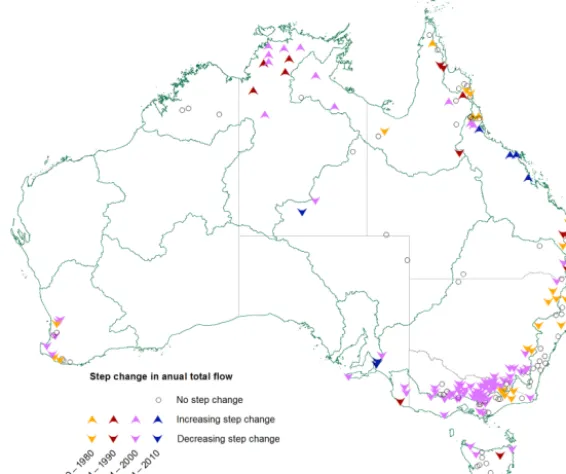
Figure 6.Variations of step change in annual total flow (QT), with the year of change indicated in each decade.

4.2.2 Step change

Step change analysis was applied to all sites where the time series data were random to give comparable results of grad-ual and abrupt changes in anngrad-ual total flows. The rank–sum test was used to identify the presence of a step change in the median of two periods, with the distribution-free CUSUM method providing the year of change. Values were reported for sites with rank–sum test at 0.1 significance levels or higher. Figure 6 shows the results of step change analysis, where colours indicate the year of change appearing in each decade and upward arrows represent increased median values after the year of change and vice versa.

The step change map reveals a definite spatial pattern in the location of stations that exhibited a significant step change. As expected, the direction and significance of step changes is consistent with the MK results for most stations. The identified years of step changes appear to show spatial groupings at different divisions. Table 2 gives the rank–sum test (RS) results and lists the year of change for the 22 sta-tions. The majority of stations in southeast Australia were characterised with step changes in the mid-1990s, when the so-called “millennium drought” (BOM and CSIRO, 2014; SEACI, 2011) started to dominate the weather in this re-gion. It has been reflected in Table 2 that 13 of 22 sta-tions presented the years of the step change in 1996, which was clearly the most dominating year. In Ummenhofer et al. (2009), where the most severe drought in Australia was discussed, the affected region referred to as southeastern Australia is defined as the land region enclosed within 35– 40◦S and 140–148◦E. Stations inside that defined region

exhibited the major feature of a step change in the 1990s which can be seen by the purple downward arrows dominat-ing Fig. 6, stations outside the region exhibited step changes with mixed years of changes. This included a good num-ber of 1970s changes at the northeast New South Wales, 1980s changes at the southeast coast of Queensland and 2000s changes in South Australia. Five stations in southwest Western Australia had a key feature of 1975 step change, which might be partly due to the observed rainfall decline since the mid-1970s. It was also noted that most stations lo-cated in the Northern Territory and some in the northeast coast of Queensland showed a significant increasing step change.

Figure 7. (a)Percentage and(b)number of stations showing significant upward and downward trends or step changes in Australian states and territories.

Mixed patterns of upward and downward step changes were detected in Queensland, which has the most diverse climatic conditions.

4.3 Spatial distribution of trends in daily flows and seasonal flows

Trend analysis maps shown in Fig. 8 decompose trends of daily flow forQMax,Q90,Q50andQ10. In general, the iden-tified trends were spatially consistent with the trend pattern inQT, with upward trends in the northwest and downward trends in the southeast, southwest and Tasmania. The Q50 and Q10 series were notable for the number stations with non-random time series and therefore an invalid MK test re-sult; this could be seen most dramatically in Fig. 8d, and was due to the higher correlation of the time series. This daily flow trend analysis indicated similar results to previous stud-ies (Tran and Ng, 2009; Durrant and Byleveld, 2009) for the respective sites and flow statistics.

The analysis of maximum daily flowQMaxcould be con-sidered as analysis of extreme flow as this series contains the maximum value for each year. The general pattern of trends inQMaxwas in accordance with the preliminary trend analysis results in Ishak et al. (2010), which suggested that about 30 % of selected stations showed trend inQMax, with downward trend in the southern part of Australia and upward trends in the northern part (Fig. 8a).

The spatial distribution of trends in seasonal flows was investigated to disaggregate total flow series into seasons (Fig. 9). The broad pattern from the analysis was a collection of few upward trends in the north and predominant down-ward trends generally in the south. Across the four seasonal variables, spring flow (QSON), winter flow (QJJA), summer flow (QDJF) and autumn flow (QMAM) were in the sequence of decreasing number of detected downward trends. All

sea-sons presented significant downward trends mostly in the southern parts of Australia, with autumn having fewer than others.

5 Discussion

We have demonstrated a comprehensive statistical and trend analysis in long-term streamflow data for 222 unregulated river gauges from the HRS national network. A total of 10 streamflow variables were examined to detect underlying changes or trend in streamflow and to identify spatial varia-tions across Australia. Evidence from previous research and this current study raises an important question: what could be the key driver of the detected changes in Australian stream-flow data? Though it is beyond scope of this study to examine underlying mechanisms linking flow, climate and other fac-tors, some remarks may help to provide valuable information for understanding and interpreting Australian hydrology.

5.1 Evidence for trends in hydrological records Australia

Figure 8.Maps showing trends of daily flow in various magnitude categories(a)maximum daily flowQMax;(b)Q90daily flow;(c)Q50 daily flow;(d)Q10daily flow at 10 % significant level (p <0.1).

at 29 sites across southwest Western Australia; they indicated the majority of sites show a consistent regional reduction in streamflow. Silberstein et al. (2012) further computed sim-ulations of runoff from 13 major river basins in southwest-ern Australia. They found that the reduction in runoff for the study region is likely to continue under projected future cli-mates. Pui et al. (2011) detected changes in annual maximum flood data of 128 stations in NSW according to multiple cli-mate drivers. Ishak et al. (2010, 2013) presented trend anal-ysis in annual maxima flood series data from 491 stations in Australia, and suggested much of the observed trend may be associated with the climate modes on annual or decadal timescales.

Commonality and differences were found from this study when compared with previous streamflow trend studies across Australia. This could be expected given the different selection of flow statistics, gauge location, data length, em-ployed techniques and methodology. For example, to

Figure 9.Maps showing trends of seasonal flow in(a)QDJFsummer flow;(b)QMAMautumn flow;(c)QJJAwinter flow;(d)QSONspring flow.

decreasing linear trend and a 1997 step change at 0.05 signif-icance level was identified in this study. No statistically sig-nificant trend was detected in Durrant and Byleveld (2009), which could be attributed to the limited record until 2008 and not considering the recent years of 2010, 2011 and 2012 that were relatively dry. The results were in agreement in both studies showing no strong decreasing trend for the Kent River at Styx Junction (604053). At this site, the 1975 change was not predominant.

The results of this study have demonstrated the main char-acterisation of hydrological change of river flows across Aus-tralia since the 1950s. Overall, most of the downward trends inQTappeared within or very close to the temperate climate zone, while upward trends were in the tropical region. Also, a large number of step changes occurred in 1996 across south-east Australia.

5.2 Further remarks on detected trends

Many factors could contribute to changes in runoff character-istics, ignoring climate change as well as low-frequency cli-mate variability and human intervention in river basins com-promise the assumption of stationarity (Ajami et al., 2016; Bayazit, 2015; Smetterm et al., 2013; Ummenhofer et al., 2009). Higher temperature and changes in precipitation or other climate variables have an impact on the rainfall–runoff process directly, and indirectly cause changes in flora, relief and soil erosion. Changes in catchment characteristics, either naturally or under human influence such as farm dams, can also have an important influence on water flow.

rivers generally have strong natural variability, subject to data availability and quality. All these factors make it challenging to detect changes or trends in streamflow data. Even if a trend is identified, it is difficult to attribute changes to any specific cause, as global warming and other regional or local changes are contributing to the hydrologic process.

The long-term rainfall trends (1970–2015) in annual total rainfall Australia has been analysed and pub-lished (http://www.bom.gov.au/climate/change/#tabs= Tracker&tracker=trend-maps). The identified trend patterns in annual total streamflow are spatially consistent with trends in annual total rainfall, where most of eastern and southwestern Australia has experienced substantial rainfall declines since 1970, while northwestern Australia has become wetter over this period. This similarity implies that hydrological variability is closely related with changes in rainfall patterns.

The spatial pattern of trends matched the rainfall records maps that indicated rainfall deficiency in the south in the last decade comparing the historical records (Cleugh et al., 2011). Similar rainfall changes were also observed as shown in the recent CSIRO sustainable yield study projects (CSIRO, 2015). Drought conditions, the most persistent rainfall deficit since the start of the 20th century, persisted in the southeast and southwest of the continent from around 1996 to 2010, which might be attributed to the detected change in stream-flow. This could be the reason that most of the gauging stations in southern Australia and southeast of Queensland showed a significant decreasing trend in annual streamflow. It was also found that positive trends observed at many loca-tions in northern Australia could be related to increased rain-fall in this part of Australia during the last decade (SEACI, 2011). Other changes such as within-year rainfall variation and increase in temperature may have played a role in affect-ing the hydrologic cycle.

Whilst it is a possible explanation, it is not explicit that cli-mate change is the only cause of significant trends in flow. There are many other factors that may affect stream-flow, for example, natural catchment changes, climate vari-ability, data artefacts and other influences. Site-specific com-parison of rainfall, PE and temperature may help to improve the understanding of the underlying causes of trends in hy-drological variables. Further investigation would be required to discover the potential causes of detected trends, which was beyond the scope of this study.

Under the Water Act (2007), the Australian Bureau of Me-teorology has responsibility for compiling and disseminating comprehensive water information nationwide. HRSs are an initial step to build up the national river data network. The network of HRSs, which the present study was based on, is the first operational website in Australia as a national river flow data repository. It provides an excellent foundation for water planning and research – particularly in trend detection and the possibility to link to large-scale atmospheric and cli-mate variables. The information on the HRS website can be

used as a test bed for model development, hydrological non-stationarity assessments and many other research interests.

6 Conclusions

This study investigated the streamflow variability and in-ferred trends in water availability for 222 gauging stations in Australia with long-term and high-quality streamflow records. The results present a systematic analysis of recent hydrological changes in greater spatial and temporal details than previously published for Australian rivers. Implications of the findings should aid decision making for water re-sources management, especially when considering the results in the context of climate variability.

The main findings of the study are

– The spatial and temporal trends in observed streamflow varied across different hydroclimatic regions in Aus-tralia (Figs. 1 and 5). As a short summary of the trend test results in annual streamflow (QT) over the conti-nent, most of the increasing trends were observed in northern part of Northern Territory, while there was only one weak trend visible in the northern region of Western Australia and Queensland. However, in south-eastern Queensland there was a significant decreasing trend. Most of the gauging stations in New South Wales, Victoria, southeast South Australia, southwest West-ern Australia and northwest Tasmania showed a signif-icant decreasing trend in annual streamflow. In central Australia, north Queensland and South Tasmania, most of the stations showed no significant trend in annual streamflow.

– The temporal trends also varied between different com-ponents of streamflow – annual total, daily maxi-mum (QMax), high, median and low flows (Q90,Q50,

Q10), baseflow (QBF) and seasonal flows (QJJA,QSON,

QDJF,QMAM). Out of 222 stations, only 7 showed an increasing trend, 90 decreasing and 98 no trend in total annual streamflow. The annual daily maximum stream-flow showed decreasing trends at 67 stations while the low flow and baseflow components showed decreasing trends at 18 and 73 stations, respectively. Trends also varied between different seasonal flows and also across different hydroclimatic regions. Seasonal flow maps were dominated with decreasing trends. A few stations in northern Australia presented increasing trend for spring, summer and winter flow, while no stations were found with increasing trend for autumn flow (QMAM) anywhere in Australia.

changes were seen in the Northern Territory and some of the northeast coast of Queensland.

– The web portal (http://www.bom.gov.au/water/hrs) dis-plays all the graphical products, tables and statistical test results of all 222 stations. It contains a comprehen-sive unique set of graphical products for linear trends and step change.

The streamflow trends evident from the statistical data anal-ysis showed some parallels with climate variability patterns that the country experienced through recent decades. Long-term trends in water availability across different hydrocli-matic regions of Australia reported in this study are derived purely from observations, not derived from models which can invariably be influenced by biases. The high-quality streamflow data of HRS and the results from this analysis on streamflow variability provide critical information for water security planning and for prioritising water infrastructure in-vestments across Australia.

7 Data availability

Appendix A: Statistical tests A1 Median crossing test

This method tests for randomness of time series data. It is a non-parametric test. The n time series values (X1, X2,

X3. . . Xn) are replaced by “0” ifXi< Xmedian and by “1”

ifXi> Xmedian. If the time series data come from a random

process, then the count “m”, which is the number of times 0 is followed by 1 or 1 is followed by 0, is approximately nor-mally distributed with

Mean: µ=(n−1)

2

Standard deviation: σ=(n−1)

4 .

Thezstatistic is therefore defined as

z=|(m−µ)|

σ0.5 .

A2 Rank difference test

This method also tests for randomness of time series data. It is a non-parametric test. The ntime series values (X1,X2,

X3. . . Xn) are replaced by their relative ranks starting from the lowest to the highest (R1, R2,R3 . . . Rn). The statis-tic “U” is the sum of the absolute rank differences between successive ranks:

U=

n

X

i=2

|Ri−Ri−1|.

For largen,Uis normally distributed with

Mean: µ=(n+1)(n−1)

3

Standard deviation: σ=(n−2)(n+1)(4n−7)

90 .

Thezstatistic∗is therefore defined as

z=|(U−µ)|

σ0.5 .

A3 Mann–Kendall test

This method tests whether there is a trend in the time series. It is a non-parametric rank-based test. Thentime series val-ues (X1,X2,X3. . . Xn) are replaced by their relative ranks starting from the lowest to the highest (R1,R2,R3. . . Rn).

The test statisticSis defined as

S=

n−1

X

i=1

" _n

X

j=i+1

sgn Ri−Rj

#

,

where

sgn(y)=1 fory >0 sgn(y)=0 fory=0 sgn(y)= −1 fory <0 sgn()is the signum function.

If there is a trend in the time series (i.e. the null hypothesisH0 is true), thenSis approximately normally distributed with Mean: µ=0

Standard deviation: σ =n(n−1)(2n+5)

18 .

Thezstatistic∗_{is therefore}

z= |S|

σ0.5.

A positive value ofS indicates that there is an increasing trend and vice versa.

A4 Distribution-free CUSUM test

This method tests whether the means in two parts of a record are different for an unknown time of change. It is a non-parametric test. Given time series data (X1,X2,X3. . . Xn), the test statisticVkis defined as

Vk=

k

X

i=1

sgn(Xi−Xmedian) ,

where

sgn(y)=1 fory >0 sgn(y)=0 fory=0 sgn(y)= −1 fory <0

Xmedianis the median value of theXidata set.

The time at which “max|Vk|” occurs is consid-ered as the time of change. The distribution of Vk follows the Kolmogorov–Smirnov two-sample statistic (KS=(2/n) max|Vk|). A negative value ofVk indicates that the latter part of the record has a higher mean than the earlier part and vice versa.

A5 Rank–sum test

Mean: µ=n(N+1)

2 Standard deviation: σ=

nm(N+1)

12

0.5

wherenandmare the number of observations in the smaller and larger groups, respectively. The standardised form of the test statistic,Z∗is computed as

Z=(S−0.5−µ)/σifS > µ

Z=0 ifS=µ

Z= |S+0.5−µ|/σ ifS < µ.

Acknowledgements. The primary streamflow data for this study were provided by the national and state water agencies. The hydro-logic reference stations website was developed in consultation with University of Melbourne, CSIRO Land and Water, Department of the Environment (DOE) and about 70 other stakeholders. Special thanks go to Emeritus Professor Tom McMahon for his contribution to the HRS technical review. We also gratefully acknowledge the input from AMDISS team, water data and Geofabric teams of the Bureau of Meteorology.

Edited by: M. Werner

Reviewed by: two anonymous referees

References

ABS – Australian Bureau of Statistics: Year Book Australia 2012, http://www.abs.gov.au/ausstats (last access: 7 August 2013), 2012.

Ajami, H., Sharma, A., Band, L. E., Evans, J. P., Tuteja, N. K., Amirthanathan, G. E., and Bari, M. A.: On the non-stationarity of hydrological response in anthropogenically unaffected catch-ments: An Australian perspective, Hydrol. Earth Syst. Sci. Dis-cuss., doi:10.5194/hess-2016-353, in review, 2016.

Australian Government: Hydrologic Reference Stations (HRS), http://www.bom.gov.au/water/hrs, last access: September 2016. Bawden, A. J., Linton, H. C., Burn, D. H., and Prowse, T. D.: A

spatiotemporal analysis of hydrological trends and variability in the Athabasca River region, Canada, J. Hydrol., 509, 333–342, 2014.

Bayazit, M.: Nonstationarity of Hydrological Records and Recent Trends in Trend Analysis: A State-of-the-art Review, Environ. Process., 2, 527–542, 2015.

Biggs, E. M. and Atkinson, P. M.: A characterisation of climate variability and trends in hydrological extremes in the Severn Up-lands, Int. J. Climatol., 31, 1634–1652, 2011.

Birsan, M. V., Molnar, P., Burlando, P., and Pfaundler, M.: Stream-flow trends in Switzerland, J. Hydrol., 314, 312–329, 2005. BOM – Bureau of Meteorology: Geospatial Data Unit: Australian

Hydrological Geospatial Fabric (Geofabric) Product Guide, Version 3.0, p. 48, http://www.bom.gov.au/water/geofabric/ documents/v3_0/ahgf_productguide_V3_0_release.pdf (last ac-cess: 15 September 2016), 2015.

BOM – Bureau of Meteorology: Annual Climate Re-port 2015, http://www.bom.gov.au/climate/annual_sum/2015/ Annual-Climate-Report-2015-LR.pdf, last access: 20 June 2016. BOM and CSIRO: State of the Climate 2014, The third report on Australia’s climate by BOM and CSIRO, http://www.bom.gov. au/state-of-the-climate (last access: 13 March 2015), 2014. Bormann, H., Pinter, N., and Elfert, S.: Hydrological signatures of

flood trends on German rivers: flood frequencies, flood heights and specific stages, J. Hydrol., 404, 50–66, 2011.

Burn, D. H. and Hag Elnur, M. A.: Detection of hydrologic trends and variability, J. Hydrol., 255, 107–122, 2002.

Chiew, F. H. S. and McMahon, T. A.: Detection of trend or change in annual flow of Australian rivers, Int. J. Climatol., 13, 643–653, 1993.

Chiew, F. H. S. and Siriwardena, L.: TREND – trend/change de-tection software, CRC for Catchment Hydrology, http://www. toolkit.net.au/trend (last access: 24 October 2014), 2005. Cleugh, H., Smith, M. S., Battaglia, M., and Graham, P. (Eds.):

Cli-mate change: science and solutions for Australia, CSIRO Pub-lishing, Australia, p. 155, 2011.

CSIRO: Reports to the Australian Government from the CSIRO Sustainable Yields Project, CSIRO, Australia, 2015.

CSIRO and BOM: Climate Change in Australia Information for Australia’s Natural Resource Management Regions, Techni-cal Report, CSIRO and Bureau of Meteorology, Australia, 222 pp., http://www.climatechangeinaustralia.gov.au/ (last ac-cess: 15 April 2016), 2015.

Dixon, H., Lawler, D. M., and Shamseldin, A. Y.: Streamflow trends in western Britain, Geophys. Res. Lett., 33, L19406, doi:10.1029/2006GL027325, 2006.

Durrant, J. and Byleveld, S.: Streamflow trends in south-west Western Australia, Surface water hydrology series – Report no. HY32, Department of Water, Government of Western Aus-tralia, p. 79, https://www.water.wa.gov.au/__data/assets/pdf_file/ 0017/1592/87846.pdf (last access: 16 September 2016), 2009. Finlayson, B. L. and McMahon, T. A.: Australia v. the world: a

com-parative analysis of streamflow characteristics, in: Fluvial Ge-omorphology of Australia, edited by: Warner, R. F., Academic Press, Sydney, 17–40, 1988.

Geoscience Australia: Australia’s River Basins 1997: Product User Guide, National Mapping Division, Geoscience Australia, Can-berra, 2004.

Haddad, K., Rahman, A., and Weinmann, P. E.: Streamflow data preparation for regional flood frequency analysis: Important Lessons from a case study, Proc. Water Down Under, 2008, 2558–2569, 2008.

Hannaford, J. and Buys, G.: Trends in seasonal river flow regimes in the UK, J. Hydrol., 475, 158–174, 2012.

Hannaford, J. and Marsh, T.: An assessment of trends in UK runoff and low flows using a network of undisturbed catchments, Int. J. Climatol., 26, 1237–1253, 2006.

Hannaford, J. and Marsh, T. J.: High-flow and flood trends in a net-work of undisturbed catchments in the UK, Int. J. Climatol., 28, 1325–1338, 2008.

Helsel, D. R. and Hirsch, R. M.: Statistical methods in water re-sources, USGS-TWRI Book 4, chap. A3, US Geological Survey, USA, 2002.

Hennessy, K., Fitzharris, B., Bates, B. C., Harvey, N., Howden, S. M., Hughes, L., Salinger, J., and Warrick, R.: Australia and New Zealand, in: Climate Change 2007: Impacts, Adaptation and Vulnerability, Contribution of Working Group II to the Fourth Assessment Report of the Intergovernmental Panel on Climate Change, edited by: Parry, M. L., Canziani, O. F., Palutikof, J. P., van der Linden, P. J., and Hanson, C. E., Cambridge University Press, Cambridge, UK, 507–540, 2007.

IPCC: Climate Change 2014, Synthesis Report, in: Contribution of Working Groups I, II and III to the Fifth Assessment Report of the Intergovernmental Panel on Climate Change, edited by: Core Writing Team, Pachauri R. K., and Meyer, L. A., IPCC, Geneva, Switzerland, 151 pp. 2014.

Environmental and Water Resources Congress 2010: Challenges of Change, 16–20 May 2010, Providence, RI, 115–124, 2010. Ishak, E. H., Rahman, A., Westra, S., Sharma, A., and Kuczera, G.:

Evaluating the non-stationarity of Australian annual maximum flood, J. Hydrol., 494, 134–145, 2013.

Jones, P. D., Lister, D. H., Wilby, R. L., and Kostopoulou, E.: Ex-tended river flow reconstructions for England and Wales, 1865– 2002, Int. J. Climatol., 26, 219–231, 2006.

Kendall, M. G.: Rank Correlation Measures, Charles Griffin, Lon-don, 1975.

Kumar, S., Merwade, V., Kam, J., and Thurner, K.: Streamflow trends in Indiana: Effects of long term persistence, precipitation and subsurface drains, J. Hydrol., 374, 171–183, 2009.

Kundzewicz, Z. W. and Robson, A.: Detecting Trend and Other Changes in Hydrological Data, World Climate Program – Wa-ter, WMO/UNESCO, WCDMP-45, WMO/TD 1013, WMO, Geneva, 158 pp., 2000.

Lins, H. F. and Slack, J. R.: Seasonal and regional characteristics of US streamflow trends in the United States from 1940 to 1999, Phys. Geogr., 26, 489–501, 2005.

Lyne, V. and Hollick, M.: Stochastic time-variable rainfall–runoff modelling, Institution of Engineers National Conference Publi-cation No. 79/10, Proceedings of the Hydrology and Water Re-sources Symposium, 10–12 September 1979, Perth, 89–93, 1979. MacDonald, N., Phillips, I. D., and Mayle, G.: Spatial and temporal variability of flood seasonality in Wales, Hydrol. Process., 24, 1806–1820, 2010.

Mann, H. B.: Non-parametric tests against trend, Econometrica, 13, 245–259, 1945.

McCabe, G. J. and Wolock, D. M.: A step increase in streamflow in the conterminous United States, Geophys. Res. Lett., 29, 2185, doi:10.1029/2002GL015999, 2002.

Miller, W. P. and Piechota, T. C.: Regional analysis of trend and step changes observed in hydroclimate variables around the Colorado River basin, J. Hydrometeorol., 9, 1020–1034, 2008.

Milly, P. C. D., Dunne, K. A., and Vecchia, A. V.: Global pattern of trends in streamflow and water availability in a changing climate, Nature, 438, 347–350, 2005.

Monk, W. A., Peters, D. L., Curry, A., and Baird, D. J.: Quanti-fying trends in indicator hydroecological variables for regime-based groups of Canadian rivers, Hydrol. Process., 25, 3086– 3100, 2011.

Nathan, R. J. and McMahon, T. A.: Evaluation of automated tech-niques for base flow and recession analyses, Water Resour. Res., 26, 1465–1473, 1990.

Novotny, E. V. and Stefan, H. G.: Stream flow in Minnesota: indi-cator of climate change, J. Hydrol., 334, 319–333, 2007. Perrin, C., Michel, C., and Andreassian, V.: Improvement of a

parsi-monious model for streamflow simulation, J. Hydrol., 279, 275– 289, 2003.

Petrone, K. C., Hughes, J. D., Van Niel, T. G., and Silberstein, R. P.: Streamflow decline in Southwestern Australia, 1950–2008, Geo-phys. Res. Lett., 37, L11401, doi:10.1029/2010GL043102, 2010. Petrow, T. and Merz, B.: Trends in flood magnitude, frequency and seasonality in Germany in the period 1951–2002, J. Hydrol., 371, 129–141, 2009.

Poff, N. L., Olden, J. D., Pepin, D. M., and Bledsoe, B. P.: Plac-ing global stream flow variability in geographic and geomorphic contexts, River Res. Appl., 22, 149–166, 2006.

Puckridge, J. T., Sheldon, F., Walker, K. F., and Boulton, A. J.: Flow variability and the ecology of large rivers, Mar. Freshwater Res., 49, 55–72, 1998.

Pui, A., Lal, A., and Sharma, A.: How does the interdecadal pacific oscillation affect design floods in Australia?, Water Resour. Res., 47, W05554, doi:10.1029/2010WR009420, 2011.

Rao, A. R., Hamed, K. H., Chen, H. L.: Nonstationarities in Hydro-logic and Environmental Time Series, in: Volume 45 of Water Science and Technology Library, Springer Science & Business Media, Springer Netherlands, 365 pp., doi:10.1007/978-94-010-0117-5, 2012.

Raupach, M. R., Briggs, P. R., Haverd, V., King, E. A., Paget, M., and Trudinger, C. M.: Australian Water Availabil-ity Project (AWAP): CSIRO Marine and Atmospheric Research Component: Final Report for Phase 3, CAWCR Technical Re-port No. 013, 67 pp., http://www.csiro.au/awap/doc/CTR_013_ online_FINAL.pdf (last access: 17 September 2016), 2009. SEACI – South Eastern Australian Climate Initiative: The

Mil-lennium Drought and 2010/11 Floods, SEACI factsheets, http://www.seaci.org/publications/documents/SEACI-2Reports/ SEACI2_Factsheet2of4_WEB_110714.pdf (last access: 17 September 2016), 2011.

Sen, P. K.: Estimates of the regression coefficient based on Kendall’s tau, J. Am.Stat. Assoc., 63, 1379–1389, 1968. Silberstein, R. P., Aryal, S. K., Durrant, J., Pearcey, M., Braccia,

M., Charles, S. P., Boniecka, L., Hodgson, G. A., Bari, M. A., Viney, N. R., and McFarlane, D. J.: Climate change and runoff in southwestern Australia, J. Hydrol., 475, 441–455, 2012. SKM: Developing guidelines for the selection of

stream-flow gauging stations. Final Report, August 2010, Pre-pared for the Climate and Water Division, Bureau of Mete-orology, 76 pp., http://www.bom.gov.au/water/hrs/media/static/ papers/SKM2010_Report.pdf (last access: 17 September 2016), 2010.

Smettem, K. R. J., Waring, R. H., Callow, J. N., Wilson, M. S. S., and Mu, Q.: Satellite-derived estimates of forest leaf area index in southwest Western Australia are not tightly coupled to inter-annual variations in rainfall: implications for groundwater de-cline in a drying climate, Global Change Biol., 19, 2401–2412, doi:10.1111/gcb.12223, 2013.

Stahl, K., Hisdal, H., Hannaford, J., Tallaksen, L. M., van Lanen, H. A. J., Sauquet, E., Demuth, S., Fendekova, M., and Jódar, J.: Streamflow trends in Europe: evidence from a dataset of near-natural catchments, Hydrol. Earth Syst. Sci., 14, 2367–2382, doi:10.5194/hess-14-2367-2010, 2010.

Stahl, K., Tallaksen, L. M., Hannaford, J., and van Lanen, H. A. J.: Filling the white space on maps of European runoff trends: estimates from a multi-model ensemble, Hydrol. Earth Syst. Sci., 16, 2035–2047, doi:10.5194/hess-16-2035-2012, 2012. Stern, H., Hoedt, G., and Ernst, J.: Objective classification of

Aus-tralian climates, Aust. Meteorol. Mag., 49, 87–96, 2000. Stewardson, M. J. and Chiew, F.: A comparison of recent trends

in gauged streamflows with climate change predictions in south east Australia, 18th World IMACS/MODSIM Congress, 13– 17 July 2009, Cairns, Australia, 2009.

Tran, H. and Ng, A.: Statistical trend analysis of river streamflows in Victoria, in: Proceedings of H2O09: 32nd Hydrology and Water Resources Symposium, 30 November–3 December 2009, Can-berra, Australia, 1019–1027, 2009.

Turner, M., Bari, M., Amirthanathan, G., and Ahmad, Z.: Aus-tralian network of hydrologic reference stations – advances in de-sign, development and implementation, 34th Hydrology and Wa-ter Resources Symposium, 19–22 November 2012, Sydney, Aus-tralia, in: Proceedings of Hydrology and Water Resources Sym-posium 2012, Engineers Australia, Barton, ACT, 1555–1564, 2012.

Ummenhofer, C. C., England, M. H., McIntosh, P. C., Meyers, G. A., Pook, M. J., Risbey, J. S., Gupta, A. S., and Taschetto, A. S.: What causes southeast Australia’s worst droughts?, Geophys. Res. Lett., 36, L04706, doi:10.1029/2008GL036801, 2009. Wang, W.: Stochasticity, Nonlinearity and Forecasting of

Stream-flow Processes, IOS Press, the Netherlands, 210 pp., 2006.

Water Act 2007: Department of Environment, Commonwealth of Australia, Start date: 3 March 2008, http://www.comlaw.gov.au/ Series/C2007A00137 (last access: 8 August 2016), 2007. WWAP – World Water Assessment Programme: The United

Na-tions World Water Development Report 4: Managing Water un-der Uncertainty and Risk, UNESCO, Paris, 2012.

Zhang, X. S., Bari, M., Amirthanathan, G., Kent, D., MacDon-ald, A., and Shin, D.: Hydrologic Reference Stations to Moni-tor Climate-Driven Streamflow Variability and Trends, 35th Hy-drology and Water Resources Symposium, 24–27 February 2014, Perth, Australia, in: Proceedings of Hydrology and Water Re-sources Symposium 2014, Engineers Australia, Barton, ACT, 1048–1055, 2014.