www.hydrol-earth-syst-sci.net/15/3253/2011/ doi:10.5194/hess-15-3253-2011
© Author(s) 2011. CC Attribution 3.0 License.
Earth System
Sciences
Recent developments in predictive uncertainty assessment based on
the model conditional processor approach
G. Coccia1,2and E. Todini1
1Department of Earth and Geo-Environmental Sciences, University of Bologna, Bologna, Italy 2Idrologia e Ambiente s.r.l., Riviera di Chiaia 72, 80122, Napoli, Italy
Received: 17 November 2010 – Published in Hydrol. Earth Syst. Sci. Discuss.: 6 December 2010 Revised: 20 October 2011 – Accepted: 23 October 2011 – Published: 28 October 2011
Abstract. The work aims at discussing the role of predictive uncertainty in flood forecasting and flood emergency man-agement, its relevance to improve the decision making pro-cess and the techniques to be used for its assessment.
Real time flood forecasting requires taking into account predictive uncertainty for a number of reasons. Determinis-tic hydrological/hydraulic forecasts give useful information about real future events, but their predictions, as usually done in practice, cannot be taken and used as real future occur-rences but rather used as pseudo-measurements of future oc-currences in order to reduce the uncertainty of decision mak-ers. Predictive Uncertainty (PU) is in fact defined as the probability of occurrence of a future value of a predictand (such as water level, discharge or water volume) conditional upon prior observations and knowledge as well as on all the information we can obtain on that specific future value from model forecasts. When dealing with commensurable quanti-ties, as in the case of floods, PU must be quantified in terms of a probability distribution function which will be used by the emergency managers in their decision process in order to improve the quality and reliability of their decisions.
After introducing the concept of PU, the presently avail-able processors are introduced and discussed in terms of their benefits and limitations. In this work the Model Conditional Processor (MCP) has been extended to the possibility of us-ing two joint Truncated Normal Distributions (TNDs), in order to improve adaptation to low and high flows.
The paper concludes by showing the results of the appli-cation of the MCP on two case studies, the Po river in Italy and the Baron Fork river, OK, USA. In the Po river case the
Correspondence to: G. Coccia
data provided by the Civil Protection of the Emilia Romagna region have been used to implement an operational exam-ple, where the predicted variable is the observed water level. In the Baron Fork River example, the data set provided by the NOAA’s National Weather Service, within the DMIP 2 Project, allowed two physically based models, the TOPKAPI model and TETIS model, to be calibrated and a data driven model to be implemented using the Artificial Neural Net-work. The three model forecasts have been combined with the aim of reducing the PU and improving the probabilistic forecast taking advantage of the different capabilities of each model approach.
1 Introduction
1.1 Decision making under uncertainty
In the last decades, the interest in assessing uncertainty in models forecasts has grown exponentially within the scien-tific communities of meteorologists and hydrologists. In par-ticular, the introduction of the Hydrological Uncertainty Pro-cessor (Krzysztofowicz, 1999; Krzysztofowicz and Kelly, 2000), aimed at assessing the predictive uncertainty in hy-drological forecasts, has created the basis for the estimation of flood predictive uncertainty.
expected value of a utility functionU (y) representing the losses, or more in general the subjective manager perception of them, as a function of a predictand that will occur at a fu-ture time (such as a fufu-ture discharge or water stage in a cross section). This quantity is unknown at the time of the decision (t0) and the aim of forecasting is to assess its probability of occurrence, in terms of a predictive uncertainty probability density function.
In the case of flood forecasting, predictive uncertainty can be defined as the uncertainty that a decision maker has on the future evolution of a predictand that he uses to make a specific decision.
In order to fully understand and to appreciate what is ac-tually meant by predictive uncertainty, it is necessary to re-alize that what will cause the flooding damages is the ac-tual future realization of the discharge and/or the water level that will occur, not the prediction generated by a forecasting model; in other words the damages will occur when the ac-tual water levelyt and certainly not if the predictionyˆt will
overtop the dyke levelyD (Todini, 2009). Therefore a util-ity/damage function at any future time (t >t0) must be ex-pressed as a function of the actual level that will occur at timet
U (yt)=0 ∀yt≤yD U (yt)=g(yt−yD) ∀yt> yD
(1) whereg(·)represents a generic function relating the cost of damages and losses to the future, albeit unknown water stage yt. In this case the manager, according to the decision
the-ory (De Groot, 1970; Raiffa and Schlaifer, 1961), must take his decisions on the basis of the expected utilityE{U (yt)}.
This value can be estimated only if the probability density function of the future event is known, and it can be written as
E{U (yt)} =
+∞
Z
0
U (yt)f (yt)dyt (2)
wheref (yt)is the probability density expressing our
incom-plete knowledge (in other words our uncertainty) on the fu-ture value that will occur. This density, which can be esti-mated from historical data, is generally too broad because it lacks the conditionality on the current events. This is why it is essential to improve this historical probability distribu-tion funcdistribu-tion by more realistically using one or more hydro-logical models able to summarize all the available informa-tion (like the rain forecast, the catchment geomorphology, the state of the river at the moment of the forecast, etc. . . ) and to provide a more informative densityf (yt|yˆt|t0), which
expresses our uncertainty on the future predictand value af-ter knowing the models’ forecasts issued at timet0, namely
ˆ
yt|t0= [ ˆy1t|t0,yˆ2t|t0,...,yˆMt|t0], where M is the number of
forecasting models. Equation (2) can now be rewritten as
E
U yt|yˆt|t0 =
+∞
Z
0
U (yt)f yt|yˆt|t0
dyt (3)
The probability distribution function f (yt|yˆt|t0) represents the PU, hereafter denominatedf (y|yˆ)for sake of simplicity. In this paper some existing uncertainty processors will be breafly discussed, focusing on the Model Conditional Pro-cessor (Todini, 2008), with particual attention to the error heteroscedasticity and the models combination, providing a solution to tackle them.
1.2 Choice of the predictand
An important issue in PU assessment is the choice of the pre-dictand. As mentioned in the previuos section, PU deals with the actual value of the variable to be predicted. To this end, it is well known that measurements are always affected by er-rors that should be taken into account. However substituting the observed value for the actual value is a common proce-dure in PU assessment even if observations do not coincide with reality. A discussion about the choice of the predictand will be carried out in this section.
It is worth to take into account the following four remarks: – Water level measurements are affected by relatively small errors (with standard error of the order of 2– 3 cm); although care should be taken to account for possible non stationarities in the records, it is psycho-logically fundamental to use them as measures unaf-fected by measurement errors both because flood deci-sions have always been essentially based on these mea-sures and because their errors have very small effect on the decisions compared to the larger effects of the other sources of uncertainty.
– Discharge measurements are generally unavailable in real time, although there is a recent tendency to use mi-crowave surface velocity measurements in combination with the water stage, which could improve discharge es-timates in real time.
– Classical discharge estimates, based on water level mea-surements and steady state rating curves, are affected by errors that may reach 30 % (Di Baldassare and Monta-nari, 2009). One major source of errors is due to ex-trapolation beyond the range of observations. A sec-ond major source is due to the presence of loops in the level-discharge relation, which are not represented by the steady state rating curve, unless modified by using correcting formulas, such as the Jones formula or others (Dottori et al., 2009).
here talking of a filtered quantity because the real occur-rence will never be known, but one can reduce the mea-surement errors by using filtering techniques aimed at re-ducing measurement errors, such as for instance the classi-cal Kalman Filtering technique (Kalman, 1960; Kalman and Bucy, 1961). Nonetheless, in practice, the observed water levels can be considered the best operational quantity to be used as predictand: the errors are small and the decision mak-ers degree of belief is very high, while this is not so for the filtered quantities that are estimated and not measured. Therefore, whenever possible, and in particular when deal-ing with flood warndeal-ing, one should use the observed water levels as the predictand to be used in any flood predictive uncertainty processor.
In case that water levels are not available or when one needs to predict inflows to a reservoir or a water detention area, where the flood volumes are the best decision vari-able, corrected and filtered discharges should be used. In other words, prior to use discharges as predictands for the calibration of the hydrological uncertainty processors, their improved estimates must be produced both by accounting for the shape of the cross section and by taking into ac-count the loop formation in the rating curve. This will elim-inate most of the water level dependent biases, while the elimination of the random errors must be approached by filtering techniques.
In terms of predictors (i.e. the variables used to condition the PU), when available from a flood routing model, the best choice would be the forecasted water levels. Otherwise it is possible either to convert the predicted discharges into pre-dicted water levels using a corrected rating curve, as men-tioned above, or just to directly use the predicted discharges, since the effect of the conversion errors from discharge to levels, may affect the order of the predicted variables. This is what essentially dominates the Normal Quantile Trans-form (NQT), which is the basis of most of the uncertainty processors (Van der Waerden, 1952, 1953a,b).
1.3 The probabilistic threshold paradigm
Today, similarly to what was done for more than a century, in order to trigger their decisions, the majority of water au-thorities involved in flood emergency management prepare their plans on the basis of pre-determined water depths or thresholds ranging from the warning water level to the flood-ing level. Decisions, and consequent actions, are then taken as soon as a real time measure of the water stage overtops one of these thresholds. This approach, which is correct and sound in the absence of flood forecasting models, is a way of anticipating events on the basis of water level measures (in the cross sections of interest or in upstream cross sections), but can only be effective on very large rivers where the time lag between the overtopping of the warning and the flooding levels is sufficiently large to allow for the implementation of the planned flood relief strategies and interventions. Given
that all the water stage measures are affected by relatively small errors (2–3 cm), they can be, and have been, considered as deterministic.
Unfortunately, the advent and the operational use of real time flood forecasting models, has not changed this ap-proach, which has been the cause of several unsatisfactory results. Today, the flood managers compare forecasts, and not the actual measurements, to the different threshold levels; this is obviously done in order to further anticipate decisions by taking advantage of the prediction time horizon. Unfortu-nately, by doing so the forecasts are implicitly assumed to be deterministic, which is not the case since they represent vir-tual reality and are affected by prediction errors, which mag-nitude is by far larger than that of the measurement errors.
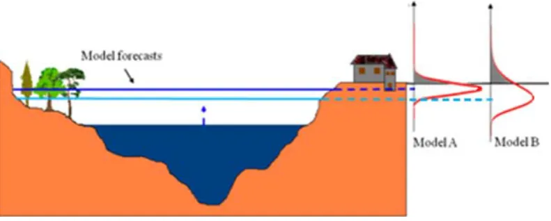
More recently, the concept of predictive uncertainty has changed this approach. This uncertain nature of forecasts, opposed to the higher accuracy of measurements, requires the definition of probabilistic thresholds, defined in terms of the probability of flooding taken at different probability lev-els, instead of the definition of deterministic threshold val-ues. Using the probabilistic thresholds, the same predicted water level may have different meaning owing to the reliabil-ity of prediction. In other words, the same forecast may or may not trigger the decision of issuing a warning or evacuat-ing an area, conditionally to its assessed level of uncertainty. More uncertain forecasts need necessarily to be treated more cautiously than more reliable ones; in fact, uncertain lower water stage forecasts could then trigger a protective measure, whereas higher, albeit more accurate water stage forecasts, would not. As can be seen from the Fig. 1, for the same expected value (the horizontal dashed line) a better forecast (Model A), characterised by a narrower predictive density, will show a smaller probability of exceeding the flooding level when compared to a worse one (Model B). This prop-erty can be also looked at from an alternative perspective, as shown in Fig. 2 the same flooding probability corresponds to lower expected values as the spread of PU increases. This implies that if a probabilistic threshold is defined instead of a deterministic threshold level, when the PU is larger the de-cision maker must be more cautious and would be advised to issue an alert even when, looking at the expected value of the forecast, he would not think of issuing it, because he may regard it as being too low.
2 Existing approaches
Fig. 1. Probability of exceeding the dyke level for the same expected value, forecasted by models with different reliability.
Fig. 2. Comparison between the expected value provided by models with different reliability when the probability of exceeding the dyke
level is the same for all the models.
2.1 Hydrological uncertainty processor
Krzysztofowicz (1999) introduced a Bayesian processor, the Hydrological Uncertainty Processor (HUP) which aims at es-timating the predictive uncertainty given a set of historical observations and a hydrological model prediction. The HUP was developed around the idea of converting both observa-tions and model predicobserva-tions into a normal space by means of the NQT in order to derive the joint distribution and the predictive conditional distribution from a treatable multivari-ate distribution. In practice, as described in Krzysztofow-icz (1999), after converting the observations and the model forecasts available for the historical period into the normal space, the HUP combines the prior predictive uncertainty (in this case derived using an autoregressive model) with a Likelihood function in order to obtain the posterior den-sity of the predictand conditional to the model forecasts. From the normal space this conditional density is finally re-converted into the real space in order to provide the predictive probability density.
[image:4.595.101.497.262.421.2]2.2 Bayesian model averaging
Introduced by Raftery (1993), Bayesian Model Averaging (BMA) has gained a certain popularity in the latest years. The scope of Bayesian Model Averaging is correctly formu-lated in that it aims at assessing the mean and variance of any future value of the predictand conditional upon several model forecasts. Differently from the HUP assumptions, in BMA all the models (including the AR prior model) are similarly considered as alternative models. Raftery et al. (2005) devel-oped the approach on the assumption that the predictand as well as the model forecasts were approximately normally dis-tributed, while Vrugt and Robinson (2007) relaxed this hy-pothesis and showed how to apply the BMA to Log-normal and Gamma distributed variables. In practice the Bayesian Inference problem, namely the need for estimating a poste-rior density for the parameters, is overcome in the BMA by estimating a number of weights via a constrained optimiza-tion problem. Once the weights have been estimated, BMA allows to estimate the mean and the variance of the predic-tand conditional upon several models at the same time.
The original BMA, as introduced by Raftery (1993), has shown several problems. First of all, as pointed out by Vrugt and Robinson (2007), the original assumption of approxi-mately normally distributed errors, is not appropriate for rep-resenting highly skewed quantities such as water discharges or water levels in rivers. Therefore one must either relax this hypothesis, as done by Vrugt and Robinson (2007) who ap-plied the BMA to Log-normal and Gamma distributed vari-ables or to convert the original in the normal space once again using the NQT, as done in Todini (2008). Another problem, which emerges from the application of BMA is the use of the “expectation-maximization” (EM) algorithm (Dempster et al., 1977) proposed by Raftery et al. (2005), which was not found to properly converge to the maximum of the likeli-hood. To overcome this problem, one can either use sophis-ticated, complex optimization tools such as the SCEM-UA (Vrugt et al., 2003) or, as proposed by Todini (2008), a sim-ple and original constrained Newton-Raphson approach, which converges in a very limited number of iterations. 2.3 Quantile regression
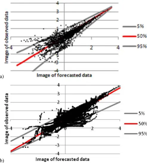
The latest uncertainty processors approaches tackle the prob-lem of the heteroscedasticity of the errors often present in hydrological modelling. All the previously described tech-niques imply homoscedasticity of the error variance, which is assumed to be independent from the magnitude of the ob-served or forecasted values, but in real cases this assumption leads to a lack of accuracy.
Recently, in order to overcome this problem, the Quantile Regression (Koenker, 2005) was used (Weerts et al., 2011). The Quantile Regression (QR) approach tries to represent the error heteroscedasticity identifying a linear or non-linear variation of the quantiles of the PU as a function of the model
forecast magnitude. This technique allows all the desired quantiles of the PU to be assessed in the normal space and then reconverted by means of the inverse NQT to the real space. In the linear case, the τ-th sample quantile is com-puted solving the Eq. (4), from which is possible to identify the parametersaτ andbτ which defines the linear regression
for theτ-th quantile. min
aτ,bτ∈R
n
X
i=1
ρτ(η−a−bτ· ˆη) (4)
where ρτ(x)=
x·(τ−1) if x <0 x·τ if x≥0
The problem is correctly formulated and allows each quan-tile of the PU to be computed, but it requires the estimation of at least two parameters per quantile and the number of parameters to be estimated may become quite large. More-over, QR not always improves from assuming homoscedas-ticity: this depends on the actual distribution of the errors. Figure 3a and b shows two situations in which the use of the linear QR leads to very different results. Figure 3a is an op-timal situation for using linear QR because the variation of error variance is linearly decreasing with the magnitude of the forecasts and the resulting quantiles well represent the real distribution of the data. On the contrary, in Fig. 3b it is not possible to identify a linear variation of the error vari-ance and the use of the linear QR does not provide improved assessments of PU, particularly for high forecast values.
3 Model conditional processor
(a)
(b)
Fig. 3. (a) An optimal situation for using the QR. (b) Poor results
are obtained using QR in the situation represented here, which, by the way, is quite common in hydrological applications.
In the Normal space the joint distribution ofηandbηcan be assumed as a Normal Bivariate,f (η,bη), allowing the predic-tive distribution to be easily computed according to the Bayes theorem, as described in (Todini, 2008). The moments of the predictive distribution in the Normal space are:
µη|bη=ρηbη
·
bη ση2|
b
η=1−ρη2bη
(5)
Therefore, after obtaining the conditional probability in the normal space, the results have to be converted into the real world in order to compute the predictive probabilityf ( y|
b y). To do so the predictive density has to be sampled in the Nor-mal space and then the obtained quantiles have to be recon-verted into the real space by a reverse process. This is due to the fact that the transformation is highly non linear, and, for instance, the mean value in the Normal space does not correspond to the mean value in the real world, in fact it cor-responds to the median (50 % probability) (Todini, 2009). In this process the use of the Weibull plotting position implies the need of using an additional model to fit to the tails of all the variables, namely the observations and the model fore-cast, in the real space, in order to accommodate probability quantiles larger than n+n1 or lower than n+11. The choice of the best tail model depends on the actual distribution of the
data, in most applications of the MCP the following models have been used, respectively for the lower and the upper tail:
p(y)=plow·
y y (plow)
a
(6)
p(y)=1− 1−pup·
"
ymax−y ymax−y pup
#b
(7)
whereplow and pup are the lower and upper limits defin-ing the probability values for which the tails will be used;y (plow)andy pup are the values of the variabley correspondent to the probability limits;ymaxis the maximum value for which the probability is assumed to be equal to 1 and, although it can be derived through an extreme value analysis, for the sake of simplicity, in the proposed case stud-ies it was assumed to be equal to twice the maximum value ever observed;a andb are the parameters to be estimated. Concerning the lower tail it is assumed that the null proba-bility is assigned to the null value of the variabley, that is true when dealing with discharges, but not if y represents level values. In this case it is necessary to refer all the val-ues to the bedstream level, so that the null level is the lowest level possible. Moreover, using level values alsoymaxmust be computed as the double of the maximum level observed referred to the bedstream level.
3.1 The multi-model case
The previously described MCP methodology has generated the idea of generalizing the procedure using a multi-normal approach (Todini, 2008). Often, a real time forecasting sys-tem is composed by more than one model, or a chain of mod-els, and the emergency manager has to take a decision on the basis of multiple forecasts of the same quantity that may also be very different from each other. It is very difficult to find an objective way to state that one model is better than another, or to assign a correct weight to each forecast in order to extrap-olate from all the available information a stochastic forecast that allows the emergency to be managed in the best way.
In order to combine several model forecasts, the MCP can be improved by generalizing the bivariate normal approach to a multivariate normal approach (Mardia et al., 1979). In this case the Multivariate space is composed byM+1 vari-ables, that are the observed discharges (or water levels) y and theM predictionsyˆk,k=1,...,M. Using the NQT, all
the variables are converted to their transformed values,ηand
ˆ
ηk,k=1,...,M, in the multi-normal space.
All the variables in the normal space have a standard nor-mal distribution and the predictive uncertainty, defined now as the distribution of the future event conditioned on the fore-casts of theM models, can be expressed as(y| ˆy1,...,yˆM),
[image:6.595.50.297.63.336.2]The joint distribution is a multi-normal distribution with mean and variance
µη,ηˆ k= 0 .. . 0 (8)
6η,ηˆk=
1 ρηηˆ1 ρηηˆ2 ··· ρηηˆM
ρηˆ1η 1 ρηˆ1ηˆ2
. .. ρ
ˆ
η1ηˆM
ρηˆ2η ρηˆ2ηˆ1
. .. . .. ... ..
. . .. . .. . .. ρηˆM−1ηˆM
ρηˆMηρηˆMηˆ1 ··· ρηˆMηˆM−1 1 (9) Defining
6ηη=1 6ηηˆ=
ρηηˆ1 ρηηˆ2 ···ρηηˆM
6ηˆηˆ=
1 ρηˆ1ηˆ2 ··· ρηˆ1ηˆM
ρηˆ2ηˆ1
. .. . .. ... ..
. . .. . .. ρηˆM−1ηˆM
ρηˆMηˆ1 ··· ρηˆMηˆM−1 1 (10)
and substituting Eq. (10) in Eq. (9), the cross correlation ma-trix can also be written as
6η,ηˆk=
"
6ηη 6ηηˆ
6ηηˆT 6
ˆ
ηηˆ
#
(11) Then the predictive uncertainty can be expressed as
f (η|ηˆk)=f (η,ηˆ1,...,ηˆM)
f (ηˆ1,...,ηˆM)
(12) The solution of Eq. (12) is easily obtained and leads to a nor-mal distribution with moments derived from Eq. (11) as
µη| ˆηk=6ηηˆ·6ηˆηˆ
−1· ˆ η1 .. . ˆ ηM σ2
η| ˆηk=1−6ηηˆ·6ηˆηˆ
−1·6 ηηˆT
(13)
Please note that Eq. (13) does not differ from the classical multiple regression results.
As done for the univariate case, the predictive uncertainty in the real world,f (y|yˆk), is obtained by convertingf (η|ηˆk) by means of the inverse NQT.
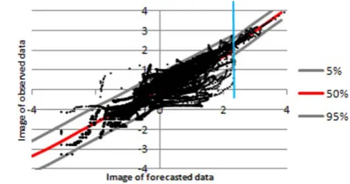
3.2 Truncated normal joint distributions to account for the error heteroscedasticity
[image:7.595.295.549.63.196.2]As mentioned in Sect. 2.3, the assumption of homoscedastic-ity of the error variance leads to a lack of accuracy in repre-senting the PU, especially at reproducing high flows, because
Fig. 4. Truncated normal joint distributions. The division of the
Joint Distribution in the normal space into two bivariate truncated normal distributions is shown. The red line represents the modal value, while the grey lines represent the 5 % and the 95 % quantiles. The light blue line represents the threshold used in order to identify the two TNDs.
the NQT tends to increase the variance of the lower values. Moreover, the number of observed and predicted low and medium flows is much larger than that of high flows with the consequence of a higher weight in the determination of the regression or the correlation coefficients used by the different approaches. As a consequence the estimation of high flows in the Normal Space will be affected by a distortion in the mean as well as an overestimation of the variance, which will in-evitably increase when returning into the real space. To face this problem an alternative approach has been introduced in the MCP formulation. Namely, within the MCP framework the entire Normal domain is divided into two (or more) sub-domains where Truncated Normal Distributions (TNDs) can be used. In this case, the MCP can be applied assuming that the joint distribution in the Normal Space is not unique, but can be divided into two (or more) TNDs. A threshold sepa-rating low flows from high flows, in the forecast domain, is relatively easy to be identified. Figure 4 shows the two TNDs that can be used in that case.
The identification of the two TNDs is not immediate, but can be obtained by the following procedure that depends on the number of available forecasting models.
3.2.1 TNDs with only one forecasting model
After converting the original variablesyandbyto their trans-formed values ηandη, a threshold a is chosen among theˆ
The threshold a can be identified as the value of ηˆ that minimizes the predictive variance of the upper sample (the one representing the high flows) and its search must be lower and upper limited in order to count with significant samples for computing the moments of the truncated distributions. In fact, the moments of these truncated distributions must be estimated by equating them to the sampling moments, as described below.
Taking into account only the sample that includes the high flows, the Truncated Normal distribution forη > aˆ is f (ηˆ| ˆη > a)= f (η)ˆ
R+∞
a f (η)dˆ ηˆ
= f (η)ˆ
1−Fηˆ(a)
(14) withf (η)ˆ defined as
f (η)ˆ =√1
2π sηˆ
exp (
−1
2 ηˆ−m
ˆ
η
sηˆ
2)
(15) wheremˆ andsˆare the mean and the standard deviation of the non truncated, albeit unknown distribution.
Therefore, the joint distribution is the following truncated normal bivariate distribution
f (η,ηˆ| ˆη > a)= f (η,η)ˆ
R+∞
−∞
h R+∞
a f (η,η)dˆ ηˆ
i dη
= f (η,η)ˆ
1−Fηˆ(a)
(16)
Wheref (η,η)ˆ is defined as
f (η,η)ˆ =
exp
−1
2
η−mηηˆ−mηˆ
S−1
η−mη
ˆ
η−mηˆ
√
2π|S| (17)
where S=
" sη2 sηηˆ
sηηˆ sη2ˆ
# .
In Eqs. (15) and (17), the values ofmηˆ,sηˆ,mη,sηandsηηˆ
are unknown but can be derived from the sampling moments. Applying the Bayes theorem to the TNDs, the predictive un-certainty becomes:
f (η| ˆη > a)=f (η,ηˆ| ˆη > a)
f (ηˆ| ˆη > a) = f (η,η)ˆ
f (η)ˆ (18)
It is normally distributed and its mean and variance are func-tional on the realization ofη,ˆ ηˆ∗> a
µη| ˆη= ˆη∗,ηˆ∗>a=mη+ sηηˆ
sηˆ2
(ηˆ∗−mηˆ)
ση2| ˆη= ˆη∗,ηˆ∗>a=s 2
η−
sη2ηˆ sη2ˆ
(19)
According to the truncated multi-normal distribution theory (Tallis, 1961), the previous equations allow the PU to be de-fined in the Normal Space as a Normal Distribution with mean and variance:
µη| ˆη= ˆη∗, bη
∗>a=µη+ σηηˆ
σηˆ2
(ηˆ∗−µηˆ)
ση2| b
η=bη∗, bη
∗>a=ση2− σηηˆ2
σηˆ2
(20)
Hereµη,µηˆ andση,σηˆ are respectively the sample means
and standard deviations ofη| ˆη > aandηˆ| ˆη > a. These mo-ments are obviously computed considering only the data included in the upper sample.
Considering now the lower sample and a relaziation ofη,ˆ ˆ
η∗< a, Eqs. (14) and (16) become, respectively
f (ηˆ| ˆη < a)= f (η)ˆ
Ra
−∞f (η)dˆ ηˆ
= f (η)ˆ
Fηˆ(a)
(21)
f (η,ηˆ| ˆη < a)= f (η,η)ˆ
R+∞ −∞[
Ra
−∞f (η,η)dˆ ηˆ]dη
=f (η,η)ˆ
Fηˆ(a)
(22)
If the same procedure carried out for the upper sample is applied to the lower sample, the predictive uncertainty is ob-tained with the following equation
µη| ˆη= ˆη∗,ηˆ∗<a=µη+ σηηˆ
σηˆ2
(ηˆ∗−µηˆ)
ση2| ˆη= ˆη∗,ηˆ∗<a=ση2− σ2
ηηˆ
σ2ˆ
η
(23)
Please note that Eq. 23 is equal to Eq. 18, but in this caseµη,
µηˆ,σηandσηˆare computed taking into account only the data
of the lower sample.
3.2.2 TNDs with more than one forecasting model When dealing with more than one model, the procedure be-comes a bit more difficult. The threshold should be identi-fied for each model and the joint distribution would be rep-resented by 2MMultivariate Truncated Normal Distributions (MTNDs) (whereMis the number of models) that include all the possible simultaneous combinations of each model over-topping or not its respective threshold. The moments of each MTNDs should be obtained by means of the sampling mo-ments computation, but unfortunately in real cases often the available data are not enough to identify representative sam-ples and the MTNDs cannot be well assessed.
In order to avoid this situation the problem can be tackled with a different approach. The MCP can be applied in three phases. Firstly, each model is processed separately using the TNDs as described above. In this phase, for each model its threshold is identified. In the second phase, the series of expected values of each model simulation (previously ob-tained) are combined again using two MTNDs. The split of the multi-variate Normal Space in two parts is obtained iden-tifying the hyperplane that includes the point[(η=0,ηˆi=
a),∀i=1..M] and is perpendicular to the straight line that links the origin to that point. This hyperplane is identified by the following equation:
M
X
i=1
ˆ
Fig. 5. The River Po catchment in Italy and the location of the gauging station of Pontelagoscuro.
The value of a is again identified as the one that mini-mizes the predictive variance of the upper sample. Finally, in the third phase the series of expected values computed in the second phase is processed using the TNDs as described in Sect. 3.2.1.
Concerning the second phase, when the valuea is identi-fied the data are split in two samples, one containing the data below the truncation hyperplane and the other above it. After computing the sampling moments for each sample, defining Hp=PMi=1ηˆiand following the truncated multi-normal
dis-tribution theory (Tallis, 1961), it can be demonstrated that the PU in the normal space, for the sample above the trun-cation hyperplane, is defined as a normal distribution with mean and variance
µη|ηˆ=ηˆ∗ ,H∗
p>M·a=µ+6ηηˆ·6ηˆηˆ
−1·(ηˆ∗
−µˆ)
ση2|ηˆ=ηˆ∗,H∗
p>M·a
=6ηη−6ηηˆ·6ηˆηˆ−1·6ηηˆT
(25)
Here µ and µˆ are, respectively the sample means of η|Hp>M·a andη|ˆ Hp>M·a and 6ηη, 6ηηˆ, 6ηˆηˆ are the
components of the covariance matrix ofη,η|ˆHp>M·a.
Considering now the sample below the truncation hyper-plane, the mean and variance of PU in normal space are
µη|ηˆ=ηˆ∗ ,H∗
p<M·a=µ+6ηηˆ·6ηˆηˆ
−1·(ηˆ∗
−µˆ)
ση2|ηˆ=ηˆ∗,H∗
p<M·a
=6ηη−6ηηˆ·6ηˆηˆ−1·6ηηˆT
(26)
Please note that Eq. (26) is equal to Eq. (25), but in this case µ,µˆ,6ηη,6ηηˆ and6ηˆηˆ are computed taking into account
only the data of the lower sample.
4 Examples of application
Two application examples will be shown in this paper in or-der to illustrate the benefits of using the proposed method-ology. The first example is an operational one, where the predictand is the observed water level. It refers to a flood forecasting system on the Po river in Italy and shows that the MCP approach is well justified for both the full or truncated normal approaches. The second example is set up in order to illustrate the benefits of using both the truncated normal ap-proach as well as the multi model apap-proach. In this case, con-cerning a recent comparison of distributed hydrological mod-els, the discharges were the only available data, while the wa-ter level data were not available. Therefore, bearing in mind the observations made in Sect. 1.2 about the predictand to be chosen, the illustration of the MCP approach and the relevant benefits is based on the solely available discharge records. 4.1 The Po river example
4.1.1 Case study and available data
real time flood forecasting and emergency management be-came extremely clear during the 2000 Po flood, as well as in the inundation of Torino in 2001. Currently a flood fore-casting system, based on the PAB hydraulic model (Todini and Bossi, 1986) combined with the Kalman Filter based al-gorithm MISP (Todini, 1978) is operational with forecast-ing horizons up to 36 h in advance. There are several river sections where flood forecasts are issued, but the most im-portant one is the ending section of the river prior to its delta where the level gauging station of Pontelagoscuro is located (Fig. 5). Flood forecasting in Pontelagoscuro is an extremely important issue because the river is here charac-terized by a suspended bed over a flat plain only protected by high earthen dykes, whose failure could cause dramatic consequences.
The data used as predictands in this work are the mea-sured water levels at Pontelagoscuro, which have been auto-matically collected in real time since 1993 by a network of telemetering gauges, while the predictors are the water level forecasts produced by the operational flood forecasting sys-tem corrected by the Kalman Filter. Nine full years of hourly data were used in this experiment, from January 2000 to De-cember 2008, in order to assess the properties of the differ-ent uncertainty processors. The complete data set has been divided in two parts, four years to calibrate the MCP and five years to validate it. All the analysis and results presented in the following sections are based on validation data.
4.1.2 Predictive uncertainty assessment
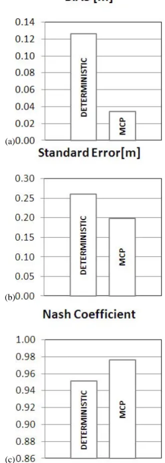
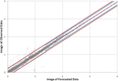
In the case of the Po river, the assessment of predictive un-certainty is made for a forecasting horizon of 36 h at Ponte-lagoscuro. Although the hydraulic model performances are quite adequate, the use of the MCP processor to provide the expected value of the predictand given the model forecasts, produces a substantial improvement by practically eliminat-ing all the bias and by reduceliminat-ing the standard error (see Fig. 6). On the contrary, in this case the use of the TNDs, instead of the standard ND, produces a rather small reduction of the un-certainty band, due to the fact that both the hypotheses on the linearity of the relation between observed and modeled nor-mal transformed variables, and on the homoschedasticity of errors, are certainly appropriate, as can be see from Fig. 7, which shows that the spread of the data is rather narrow and more or less constant over the entire field. Nonetheless the use of the TNDs slightly reduces the standard error of high water levels as can be seen in Fig. 8.
4.1.3 Probability of exceeding an alert threshold assessment
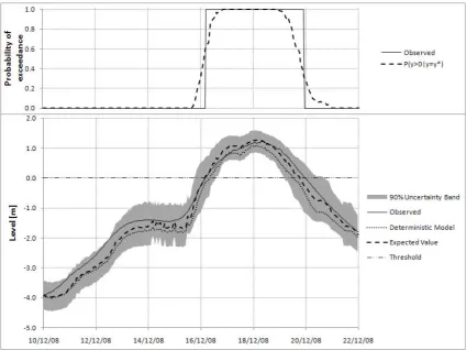
As can be seen from Fig. 9, a rather effective operational de-cision supporting tool can be set up by setting the probability threshold at 0.5. Fig. 9 shows an example of 36 h in advance prediction, during the validation period, when the water level
(a)
(b)
[image:10.595.344.509.73.536.2](c)
Fig. 6. Comparison between the evaluation indexes for the
deter-ministic model and those obtained from the PU expected value pro-vided by the MCP for the entire validation period. (a) Bias; (b) Standard Error; (c) Nash-Sutcliffe coefficient.
Fig. 7. Representation of the Normal Space obtained applying the MCP to the Po river. The full red lines represent the 5 % and 95 % quantiles
and the dashed red line the 50 % quantile obtained without using the TNDs methodology. The blue lines represent the quantiles obtained using the TNDs methodology.
Fig. 8. Zoom of the high values shown in Fig. 7. The full red lines represent the 5 % and 95 % quantiles and the dashed red line the 50 %
[image:11.595.99.503.394.666.2]Fig. 9. Flood event for the validation period predicted 36 h in advance. The lower panel represents the level forecast; observed values
(continuous line); deterministic forecast (dotted line); expected value conditioned to the model forecast (dashed line); 90 % uncertainty band (grey area); and alarm threshold of 0 m (horizontal dashed line). The upper panel represents the probability of exceeding the alarm threshold; observed binary response (continuous line) and probability of exceeding the threshold computed by the MCP (dashed line).
[image:12.595.81.506.463.688.2](a)
(b)
[image:13.595.125.474.55.686.2](c)
(a)
[image:14.595.48.288.61.319.2](b)
Fig. 12. Evaluation indexes for TOPKAPIi model (TPK), TETIS
model (TET), ANN model and their combinations during the entire validation period of the MCP. (a) Standard Error; (b) Nash-Sutcliffe coefficient.
the probability of exceeding the threshold computed using the MCP approach (dashed line). It can be seen that all the forecasts are quite adequate in this example while the proba-bility of exceeding the threshold takes values larger than 0.5, closely matching the observed binary response.
4.2 The Baron Fork river example 4.2.1 Case study and available data
The NOAA’s National Weather Service, has provided a long series of observed discharge and precipitation data for the Baron Fork River, OK (USA) within the frame of the DMIP 2 Project. Using this data set three models were imple-mented: two physically based hydrological models, the TOP-KAPI model (Todini and Ciarapica, 2001; Liu and Todini, 2002) and TETIS model (Franc´es et al., 2007; Velez et al., 2009), and a data driven model based on Artificial Neu-ral Networks. The catchment has a drainage area of about 800 km2at the measurement station of Eldon with a concen-tration time of approximately 10 h and a mean slope around 0.25 %. Some kilometers downstream Eldon the river flows into the Illinois river. The simulations provided by the three models have been processed using the MCP, firstly each model separately and then combining them.
The available meteorological data consisted in hourly rain and temperature grids with a 4 km resolution between
1 October 1995 and 30 September 2002. During the same period, also the observed discharges at the measurement sta-tion of Eldon were available. Concerning the available data, it is worth mentioning that no water level or rating curve ob-servations were available to the participants involved in the DMIP2 Project. For this reason, the discharge has been used as predictand.
4.2.2 The real time flood forecasting models
The TOPKAPI model has been developed at the University of Bologna (Todini and Ciarapica, 2001; Liu and Todini, 2002), it is composed of six components that take into ac-count the surface, sub-surface and deep flows, the channel routing, the snow accumulation/melt and the evapotranspi-ration processes. The application domain is divided in cells where the mass and momentum balance are solved at every time step. The model has been calibrated by a trial and error procedure considering the period between 1 October 1996 and 30 September 2002; the year included between 1 Octo-ber 1995 and 30 SeptemOcto-ber 1996 has been used as “warm up” period, allowing the model to reach a reasonable initial state. In the TETIS model, developed by the Polytechnic Uni-versity of Valencia (Franc´es et al., 2007; Velez et al., 2009), the conceptual scheme, at each cell, consists of a series of 5 connected tanks, each one of them representing different water storages in the soil column. The vertical connections between tanks describe the precipitation, evapotranspiration, infiltration and percolation processes, whereas, the hor-izontal flows represent the main hydrological processes as: snowmelt, overland runoff, interflow and base flow. The routing along the channel network couples its geomorpho-logic characteristics with the kinematic wave approach. The TETIS model has an automatic calibration procedure that has been used to calibrate the model considering the hydrological year included between October 2000 and September 2001. Also for the TETIS model, the first year of data has been used as “warm up” period and with the remaining data the model has been validated.
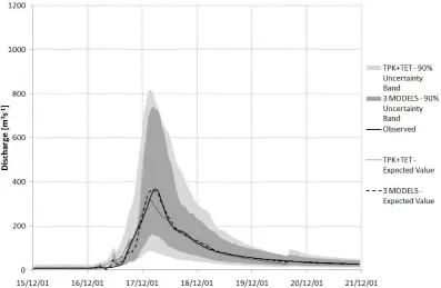
Fig. 13. Comparison between the PU computed with one or two models on a flood event for the calibration period. Observed discharges
(black line); expected value conditioned only to the TOPKAPI forecast (dashed line); expected value conditioned to the TOPKAPI and TETIS forecasts (dotted line); 90 % uncertainty band conditioned to the TOPKAPI forecast (light grey band); 90 % uncertainty band conditioned to the TOPKAPI and TETIS forecasts (grey band).
Fig. 14. Comparison between the PU computed combining, two or three models on a flood event for the calibration period. Observed
[image:15.595.99.497.391.650.2]Fig. 15. Comparison between the PU computed with one or two models on a flood event for the validation period. Observed discharges
(black line); expected value conditioned only to the TOPKAPI forecast (dashed line); expected value conditioned to the TOPKAPI and TETIS forecasts (dotted line); 90 % uncertainty band conditioned to the TOPKAPI forecast (light grey band); 90 % uncertainty band conditioned to the TOPKAPI and TETIS forecasts (grey band).
Fig. 16. Comparison between the PU computed combining, two or three models on a flood event for the validation period. Observed
[image:16.595.101.497.400.658.2]Table 1. Probability that the true value exceeds the 350 m3s−1 threshold when the expected value of prediction equals 250 m3s−1, computed for each model and their Bayesian combination.
P (y>350 m3s−1| ˆy=250 m3s−1)
TOPKAPI TETIS ANN 3 MODELS
0.25 0.34 0.16 0.15
the observed discharges during 3 h beforet0. The output of the networks is the discharge 6 h after thet0. Summarizing, the data have been divided in three groups using the SOM, in order to identify three different hydrological states of the system, and each group has been calibrated with a Feed For-ward Network in order to forecast the discharge 6 h in ad-vance. Moreover, to avoid the risk of overfitting the calibra-tion data, an early stopping procedure has been used intro-ducing a verification data set, included between 1 June 1997 and 31 January 1998. This procedure stops the Neural Net-work calibration as soon as the evaluation indexes computed on the verification data set starts to decrease. Finally, the data included between 1 February 1998 and 30 September 2002 have been used for validating the model.
In order to make coherent the forecasts of each model also the TETIS and TOPKAPI models have been used to pre-dict the discharge 6 h in advance, assuming, as done with the ANN, that the precipitation is null during the forecast time.
In Fig. 10 a schematic summary of the division of the data used for calibrating and validating each model is depicted.
The two physically based models are conceptually quite similar; it can be highlighted that the TOPKAPI model tends to underestimate the highest flood events, to overestimate the smallest ones and to reproduce the flood events of medium magnitude quite well. The TETIS model also generally un-derestimates the highest events and often unun-derestimates the small events too. The ANN model, due to its nature of data driven model, is not able to well reproduce the peak flows, which are often underestimated and predicted with a delay of 1 or 2 h, but it perfectly reproduces the low flows. 4.2.3 Predictive uncertainty assessment
The MCP is applied in three phases and Joint TNDs have been used in each phase.
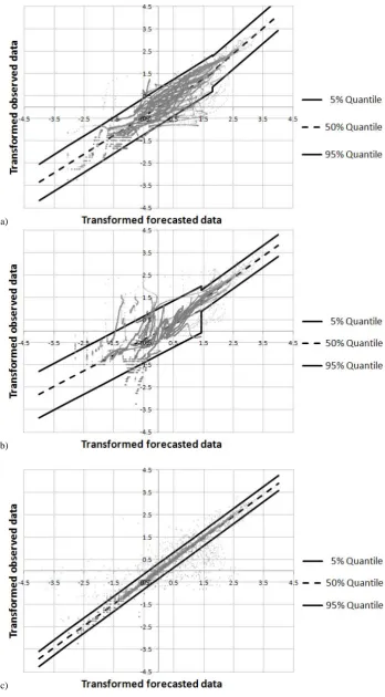
1. In the first step, each model is processed separately. All the historical data are being processed and the expected value of the predictand conditional to a single model is computed at each time step from the predictive distribu-tion. Figure 11a, b and c, schematically represents the predictive distribution computed separately with each model. For the ANN model it was not necessary to di-vide the data in two samples because the joint distribu-tion of observed and forecasted transformed values was
well represented by just a single bi-variate normal dis-tribution. The TNDs have been used for the other two models and both of them provide a lower uncertainty for the upper sample.
2. In the second step, the series of the expected values of the predictand conditional on each model forecast is processed with the MCP multivariate approach and the combined expected value of the predictand conditional to all the models is computed at each time step from the predictive distribution.
3. In the third step, the series of expected values of the pre-dictand conditional to all the models is finally processed in order to properly estimate the predictive density. This last step is required, as it will be discussed in the next section, due to the non perfect agreement between the empirical density of residual and the assumed Normal distribution.
Figure 12a and b summarizes the obtained results with re-gard to the models combination computed from the expected value of the predictive distribution. Figure 12a represents the standard error and Fig. 12b represents the Nash-Sutcliffe coefficient.
In Figs. 13, 14 and 15, 16 two examples of models com-bination are shown, one during the calibration period and the other one during the validation period. In both events the uncertainty band gets narrower as the number of models in-creases and in the calibration event the expected value com-puted with the combination of all the models well matches the observed series. In the validation event, the pick flow is quite better represented when only the TOPKAPI model is used, probably due to its better forecast in this specific case, but also in this event the uncertainty band is reduced combining all the models.
The combination of the three models’ predictions, ob-tained by assigning different weights to each model accord-ing to the Bayesian theory, allows the forecast quality to be improved as shown by the evaluation indexes in Fig. 12a and b. The two physically based model structures are very similar, so this leads to a little gain in terms of forecast im-provement, represented by the standard deviation of the er-rors and the Nash-Sutcliffe efficiency index (Fig. 12a and b). On the contrary, the combination of one physically based model with the data driven model leads to greater improve-ments in forecast and, in particular, the combination of all the three models gives the best values of the analyzed indexes (Fig. 12a and b).
Fig. 17. Flood event for the calibration period. The lower panel represents the discharge forecast; observed values (continuous line);
ex-pected value conditioned to the TOPKAPI, TETIS and ANN forecasts (dashed line); 90 % uncertainty band (grey area); alarm threshold of 350 m3s−1(small dashed line). The upper panel represents the probability of exceeding the alarm threshold; observed binary response (continuous line) and Probability of exceeding the threshold computed by the MCP (dashed line).
[image:18.595.320.536.549.595.2]It has been also shown that the combination of several models leads to improved estimation of such exceeding prob-ability. Tables 1 and 2 exemplify the improvements ob-tainable by the Bayesian combination of the different mod-els. Table 1 concurs with the behaviour represented in Fig. 1 showing the probability that the true value exceeds the 350 m3s−1threshold when the expected value of predic-tion equals 250 m3s−1, computed for each model and their Bayesian combination. One can see the reduction of ex-ceedance probability as a function of the quality of the fore-cast. Finally, the effect of the introduction of the probabilis-tic forecast approach can be appreciated in Table 2. It shows, similarly to what is qualitatively displayed in Fig. 2, the ex-pected value of the prediction corresponding to the probabil-ity of 20 % to exceed the 350 m3s−1 threshold; this value is computed for each model and for their Bayesian com-bination. As can be seen better models allow to wait un-til the expected value of prediction is closer to the flooding
Table 2. Expected value of prediction corresponding to the
proba-bility of 20 % that the true value will exceed the 350 m3s−1 thresh-old, computed for each model and their Bayesian combination.
E[y| ˆy]|[P (y>350 m3s−1| ˆy)=0.2]
TOPKAPI TETIS ANN 3 MODELS
217 m3s−1 138 m3s−1 270 m3s−1 284 m3s−1
Fig. 18. Flood event for the validation period. The lower panel represents the discharge forecast; observed values (continuous line);
ex-pected value conditioned to the TOPKAPI, TETIS and ANN forecasts (dashed line); 90 % uncertainty band (grey area); alarm threshold of 350 m3s−1(small dashed line). The upper panel represents the probability of exceeding the alarm threshold; observed binary response (continuous line) and Probability of exceeding the threshold computed by the MCP (dashed line).
4.2.4 Quantiles assessment
As mentioned in the previous section, in order to obtain a more adherent representation of the predictive density, which is essential for decision making, a third step was deemed nec-essary in the procedure after analyzing the residuals of the second step. The probability distribution of these residuals, although appearing reasonably well represented by a Nor-mal distribution in the central portion, showed high kurtosis values due to fatter tails, which induced overestimating the predictive variance under the Normal Distribution assump-tion. Due to the fact that decisions in flood management are essentially based on probabilities in the range 0.1–0.9 (one must realize that 0.9 probability of overtopping a threshold is already extremely high when taking decisions) it was de-cided that the estimation of the full predictive density would be based on a reduced set of data: namely all the couples of observation-expected value of the predictand conditional to all the models, that would generate a residual falling into the probability range 0.1–0.9. Therefore, in the third step, the application of MCP was based on this reduced set of data only, and the results were quite rewarding even in the case
(a)
[image:20.595.312.560.62.381.2](b)
Fig. 19. Comparison between the empirical distribution of residuals
and the assumed Normal distribution (σ=0.072). The results were obtained considering the entire calibration (a) and verification (b) periods for the bayesian combination of the three models.
5 Conclusions
This paper is focused on the Model Conditional Proces-sor (Todini, 2008) development for assessing predictive un-certainty. Two applications, the first one to the Po River (Italy) and the second one to the Baron Fork River (OK, USA), allowed to draw some important conclusions, which are summarized below.
The predictive uncertainty assessment starts with the iden-tification of the marginal distributions of the observed and predicted data as well as their joint distribution. Such marginal distributions are often unknown in the untrans-formed observation space, and moreover it is extremely dif-ficult to make hypotheses on the shape of their joint distribu-tion. Several works in the literature (Krzysztofowicz, 1999; Montanari and Brath, 2004; Todini, 2008) suggested to use a non-parametric approach based on order statistics, namely to use the Weibull Plotting Position as an estimate of the prob-ability of an ordered vector. Accordingly, a nonlinear trans-formation, the Normal Quantile Transform, is used to move from the original observation space to the Normal one, where
(a)
(b)
Fig. 20. Percentage of observed data that fall inside the uncertainty
band at various probability levels defined with a 10 % interval. The red line represents the perfect behaviour. The results were obtained considering the entire calibration (a) and verification (b) periods for the bayesian combination of the three models.
by construction the marginal distributions assume a Standard Normal shape and the joint distribution can be reasonably ap-proximated by a Multivariate Normal distribution. Nonethe-less, this approach has some disadvantages. First of all, it implies to identify additional models to adjust the quantiles outside the range of the historical available data. The pro-posed technique is quite sensitive to the shape and to the pa-rameters of these models and some precautions in the choice of the subset of observations used for calibrating the tails data must be taken. They must contain a large variety of cases, as required by any Bayesian approach, and in order to reduce the uncertainty on the marginal distribution tails the calibra-tion data must include the highest number of extreme cases.
[image:20.595.46.294.66.389.2]Normal joint distributions. This technique can be easily de-veloped and applied obtaining good results such as for the study cases where it has been used. The results shown in Fig. 20 demonstrate that the joint distribution is well rep-resented with this technique, even if some unavoidable ap-proximations are still present. Nevertheless, the methodol-ogy should be tested considering other catchments with dif-ferent features and for each specific application the correct-ness of the joint distribution representation must be verified. However, it must be noted that the use of the TNDs does not affect those cases when the data are homoscedastically dis-tributed, as shown in Figs. 8 and 11c, but it helps to take into account the heteroscedasticity when it is present, as shown in Fig. 11a and b.
Nevertheless, the TND assumption for the joint distribu-tion showed to be not fully correct; in fact, under the hypoth-esis of Normality, the residuals should be distributed accord-ing to a Normal distribution. In the case of the Baron Fork river, they showed to be Normally distributed in the central portion, but also to have a high kurtosis due to their fat tails. This problem can be reasonably solved in the last phase of the MCP application taking into account just the data that provide residuals inside the 0.1–0.9 probability band. Fig-ures 19 and 20 confirmed the correctness of PU assessment, at least for probability values included inside the 80–90 % around the expected value of the predictand.
Multiple predictions originated by several models, as dis-cussed in the introduction, is of difficult understanding and interpretation by the decision makers. The application of the MCP to the Baron Fork river has shown that this technique allows the correct combination of different forecasts into an unique probability of the event, which is of much easier inter-pretation and use in the decision making process. Moreover, the obtained results show that the combination of models of different nature allows the probabilistic forecast to improve the deterministic forecast of each model, taking advantage of the benefits of different hydrological approaches.
With this work, a discussion about the convenience of us-ing a probabilistic threshold instead of a deterministic one in order to estimate the flooding risk and help the decision mak-ing process about givmak-ing or not a flood alarm, has been ini-tiated. When hydrological forecasts can be defined in terms of a binary response (i.e. being below or above a threshold or giving or not a flood alarm) the probabilistic threshold concept allows the reliability and the information provided by different models to be taken into account in a combined and unique probability level. Therefore, the emergency man-ager can express his/her propensity to the risk in terms of probability of flooding and not just comparing a pre-fixed real threshold with the model forecast (which is nothing else than virtual reality), as usually done with the deterministic approach. In this respect, the paper also highlighted the need for a change in flood forecasting and warning approaches with the definition of probabilistic thresholds which aim at taking advantage of probabilistic forecasts in a more effective
way. The results presented in Sect. 4.2.4 show the good per-formance of the methodology at correctly assessing the quan-tiles up to 80–90 % around the expected value of the predic-tand, which then allows a decision maker to correctly infer the probability of exceeding an alarm threshold or a dyke.
Acknowledgements. This work was supported by the Italian Ministry of Education. The authors thank C. Mazzetti and M. Martina for their guidance and advices. G. C. would like to thank J. C. Munera and F. Franc´es for providing the results and explanations of the TETIS model. G. C. also thanks L. Pujol and Hidrogaia S. L. for the support in developing the Artificial Neural Networks Model. Finally, the authors thank the Civil Protection of Emilia Romagna Region and the NOAA’s National Weather Service for providing the data used in the study cases.
Edited by: K. Bishop
References
De Groot, M. H.: Optimal Statistical Decision, McGraw-Hill, New York, 1970.
Dempster, A. P., Laird, N. M., and Rubin, D. B.: Maximum like-lihood from incomplete data via the EM algorithm, J. Roy. Stat. Soc. B, 39, 1–39, 1977.
Di Baldassarre, G. and Montanari, A.: Uncertainty in river dis-charge observations: a quantitative analysis, Hydrol. Earth Syst. Sci., 13, 913–921, doi:10.5194/hess-13-913-2009, 2009. Dottori, F., Martina, M. L. V., and Todini, E.: A dynamic rating
curve approach to indirect discharge measurement, Hydrol. Earth Syst. Sci., 13, 847–863, doi:10.5194/hess-13-847-2009, 2009. Franc´es, F., Velez, J. I., and Velez, J. J.: Split-parameter structure for
the automatic calibration of distributed hydrological models, J. Hydrol., 332, 226–240, 2007
Kalman, R. E.: A new Approach to linear filtering and prediction problems. J. Basic Eng. Trans. ASME, 82 D, 35–45, 1960. Kalman, R. E. and Bucy, R. S.: New results in linear filtering and
prediction theory. J. Basic Eng. Trans. ASME, 83 D, 95–108, 1961.
Kennedy, M. C. and O’Hagan, A.: Bayesian calibration of computer models, J. Roy. Stat. Soc. B., 63, 425–450, 2001.
Koenker, R.: Quantile Regression, Econometric Society Mono-graphs, Cambridge University Press, New York, NY, 2005. Kohonen T.: The self-organizing map, P. IEEE, 78, 1464–1480,
doi:10.1109/5.58325, 1990.
Krzysztofowicz, R.: Bayesian theory of probabilistic forecasting via deterministic hydrologic model, Water Resour. Res., 35, 2739–2750, 1999.
Krzysztofowicz, R. and Kelly, K. S.: Hydrologic uncertainty pro-cessor for probabilistic river stage forecasting, Water Resour. Res., 36, 3265–3277, 2000.
Liu, Z. and Todini, E.: Towards a comprehensive physically-based rainfall-runoff model, Hydrol. Earth Syst. Sci., 6, 859–881, doi:10.5194/hess-6-859-2002, 2002.
Montanari, A. and Brath, A.: A stochastic approach for assessing the uncertainty of rainfall-runoff simulation, Water Resour. Res., 40, W01106, doi:10.1029/2003WR002540, 2004
Parker, D. B.: Optimal algorithms for adaptive networks: Second order backpropagation, second order direct propagation and sec-ond order Hebbian learning, IEEE 1st Int. Conf. Neural Net-works, 2, 593–600, 1987.
Pujol, L.: Prediccion de caudales en tiempo real en grandes cuencas utilizando redes neuronales artificiales, Ph.D. dissertation, Poly-technic University of Valencia, Department of Hydraulic Engi-neering and Environment, 34–39, 126–134, 2009.
Raftery, A. E.: Bayesian model selection in structural equation models, in: Testing Structural Equation Models, edited by: Bollen, K. A. and Long, J. S., Sage, Beverly Hills, CA, 163–180, 1993.
Raftery, A. E., Balabdaoui, F., Gneiting, T., and Polakowski, M.: Using Bayesian model averaging to calibrate forecast ensembles, Mon. Weather Rev., 133, 1155–1174, 2005.
Raiffa, H. and Schlaifer, R.: Applied Statistical Decision Theory, The MIT Press, Cambridge, 1961.
Tallis, G. M.: The moment generating function of the truncated multi-normal distribution, J. Roy. Stat. Soc. B, 23, 223–229, 1961.
Todini E.: Mutually Interactive State/Parameter Estimation (MISP), in: Application of Kalman Filter to Hydrology, edited by: Chao-Lin Chiu, Hydraulics and Water Resources, University of Pitts-burgh, Penn, 1978.
Todini, E.: A model conditional processor to assess predictive un-certainty in flood forecasting, Int. J. River Basin Manage., 6, 123–137, 2008.
Todini, E.: Predictive uncertainty assessment in real time flood fore-casting, edited by: Baveye, P. C., Laba, M., and Mysiak, J., Un-certainties in Environmental Modelling and Consequences for Policy Making, NATO Science for Peace and Security Series C: Environmental Security, Springer Netherlands, Amsterdam, NL, 205–228, doi:10.1007/978-90-481-2636-1 9, 2009.
Todini, E. and Bossi, A.: PAB (Parabolic and Backwater) an Uncon-ditionally Stable Flood Routing Scheme Suited for Real-Time Forecasting and Control, J. Hydraul. Res., 24, 405–424, 1986.
Todini, E. and Ciarapica, L.: The TOPKAPI model, in: Mathemat-ical Models of Large Watershed Hydrology, chap. 12, edited by: Singh. V. P., Water Resources Publications, Littleton, 2001. Van der Waerden, B. L.: Order tests for two-sample problem and
their power I, Indagat. Math., 14, 453–458, 1952.
Van der Waerden, B. L.: Order tests for two-sample problem and their power II, Indagat. Math., 15, 303–310, 1953a.
Van der Waerden, B. L.: Order tests for two-sample problem and their power III, Indagat. Math., 15, 311–316, 1953b.
V´elez, J. J., Puricelli, M., L´opez Unzu, F., and Franc´es, F.: Param-eter extrapolation to ungauged basins with a hydrological dis-tributed model in a regional framework, Hydrol. Earth Syst. Sci., 13, 229–246, doi:10.5194/hess-13-229-2009, 2009.
Vrugt, J. A. and Robinson, B. A.: Treatment of uncertainty using ensemble methods: Comparison of sequential data assimilation and Bayesian model averaging, Water Resour. Res., 43, W01411, doi:10.1029/2005WR004838, 2007.
Vrugt, J. A., Gupta, H. V., Bouten, W., and Sorooshian, S.: A Shuf-fled Complex Evolution Metropolis Algorithm for optimiza-tion and uncertainty assessment of hydrological model parame-ters, Water Resour. Res., 39, 1201, doi:10.1029/2002WR001642, 2003.
Weerts, A. H., Winsemius, H. C., and Verkade, J. S.: Estima-tion of predictive hydrological uncertainty using quantile regres-sion: examples from the National Flood Forecasting System (England and Wales), Hydrol. Earth Syst. Sci., 15, 255–265, doi:10.5194/hess-15-255-2011, 2011.
Werbos, P.: Beyond Regression: New Tools for Prediction and Analysis in the Behavioral Science, Ph. D. dissertation, Harvard University, Cambridge, 1974.
Werbos, P.: Generalization of backpropagation with application to a recurrent gas model, Neural Networks, 1, 339–356, 1988. Werbos, P.: Backpropagation through time: What it does and how