www.hydrol-earth-syst-sci.net/16/3659/2012/ doi:10.5194/hess-16-3659-2012
© Author(s) 2012. CC Attribution 3.0 License.
Earth System
Sciences
An algorithm for generating soil moisture and snow depth maps
from microwave spaceborne radiometers: HydroAlgo
E. Santi, S. Pettinato, S. Paloscia, P. Pampaloni, G. Macelloni, and M. Brogioni
CNR-IFAC, Via Madonna del Piano, 10, 50019 Firenze, Italy Correspondence to: E. Santi ([email protected])
Received: 10 February 2012 – Published in Hydrol. Earth Syst. Sci. Discuss.: 27 March 2012 Revised: 7 September 2012 – Accepted: 18 September 2012 – Published: 16 October 2012
Abstract. A systematic and timely monitoring of land sur-face parameters that affect the hydrological cycle at local and global scales is of primary importance in obtaining a better understanding of geophysical processes and in man-aging environmental resources as well as natural disasters. Soil moisture and snow water equivalent are two quantities that play a major role in these applications. In this paper an algorithm for hydrological purposes (called hereinafter Hy-droAlgo), which is able to generate maps of snow depth (SD) and soil moisture content (SMC) from AMSR-E data, has been developed and implemented within the framework of the JAXA ADEOS-II/AMSR-E and GCOM/AMSR-2 pro-grams, as well as of a project of the Italian Space Agency that is devoted to civil protection from floods and landslides. As auxiliary output, the algorithm also generates maps of vegetation biomass (VB). An initial phase of pre-processing includes the improvement of spatial resolution, as well as masking for urban areas, water bodies, and dense vegetation. The algorithm was then split into two branches, the first of which focused on the retrieval of SMC and the second, on SD. Both parameters were retrieved using Artificial Neural Network (ANN) methods. The algorithm was calibrated us-ing a wide set of experimental data collected on three sites: Mongolia and Australia (for SMC), and Siberia (for SD), in-tegrated with model simulations. These results were then val-idated by comparing the algorithm outputs with experimental data collected on two additional sites: a part of a watershed in Northern Italy, and a large portion of Scandinavia. An ad-ditional test of the algorithm was also performed on a large scale, and included sites characterized by differing climatic and meteorological conditions.
1 Introduction
The number of weather-related natural disasters, such as floods, storms, cyclones, drought and extreme temperatures, is dramatically increasing, resulting in human and economic losses which strike at least one third of the world’s pop-ulation. Such disasters are primarily due to environmental change and land degradation, which are mostly caused by human impact on the territory (e.g. Bates et al., 2008).
with onboard sensors for global surveillance and the retrieval of information regarding the Earth’s conditions.
Several major ongoing projects focus on estimating the most important parameters of the hydrological cycle. These include the AQUA/AMSR-E (Advanced Microwave Scan-ning Radiometer for EO) of NASA (National Aeronautics and Space Administration) and JAXA (Japan Aerospace Ex-ploration Agency) (Kawanishi et al., 2003), the ESA Soil Moisture and Salinity Mission (SMOS) (Kerr et al., 2010), as well as the future Soil Moisture Active Passive (SMAP) of NASA (Edelstein et al., 2010), which is the follow-up to an initial project called Hydros, and the Global Change Observation Mission–Water (GCOM-W/AMSR-2) of JAXA (Shimoda, 2009). An interesting survey of these projects was published in a recent Special Issue of PIEEE (Tsang and Jackson, 2010). In Italy, the PROSA (Products of Earth Observation for the Meteorological Alert) national project, funded by the Italian Space Agency (ASI), aimed to con-tribute to civil protection from floods and landslides by de-veloping a series of products derived from microwave and optical satellite sensors (Pettinato et al., 2009). During such emergencies, these products enable immediate assessment of the areas at risk, and/or provide support in the decision-making process regarding relief and clean-up operations. Generations of real time SMC and SD maps from passive microwave sensors are the key outputs of this project.
Research enabling the retrieval of SMC and SD from sin-gle or multifrequency radiometric data dates back to the late 1970’s, when several investigations indicated microwave emission sensitivity to SMC and SWE (e.g. Njoku and Kong, 1977; Ulaby and Stiles, 1980; Hofer and M¨atzler, 1980; Shutko, 1982; Jackson et al., 1982; Chang et al., 1982). Al-though microwave radiometers from space have a coarse ground resolution, they are able to produce daily maps of brightness temperature (Tb), which can then be converted to
SMC and SD by using appropriate inversion algorithms (e.g. Shibata et al., 2003; Njoku et al., 2003; Kelly et al., 2003).
Measurements at frequencies between 1 and 3 GHz (L band) are best suited for SMC detection, because energy is emitted from a deeper soil layer and less energy is at-tenuated by vegetation (e.g. Shutko, 1982; Paloscia et al., 1993). The SMOS mission, which is specifically dedicated to the estimating of SMC, is currently operating at 1.4 GHz (Barre et al., 2008). However, there is potential in retrieving SMC from space-borne instruments at higher frequencies, as demonstrated in over ten years of research on the sensitivity of emission at C-band (which is the lowest frequency channel available from AMSR-E) to moisture of low vegetated soils (e.g. Vinnikov et al., 1999; Jackson and Hsu, 2001; Macel-loni et al., 2003). This higher frequency band has the advan-tage of being less affected by the Radio Frequency Interfer-ences (RFI), which may severely limit the proper functioning of L-band systems (Skou et al., 2010; Balling et al., 2010). RFI can be a serious problem, especially on densely popu-lated areas, as it affects different frequencies depending on
the country. For example, C-band data are significantly con-taminated in the US, Japan and the Middle East, so that some algorithms for the retrieval of SMC employ higher frequency data despite the higher sensitivity to vegetation and surface roughness. In Europe, the problem is just the opposite, since X-band data have been found to be the ones most affected by RFI (Njoku et al., 2005).
Several approaches for the retrieval of SMC from single or multifrequency radiometric data have been investigated in previous studies. Most of these studies (Njoku et al., 2000, 2003; Jackson, 1993; Wigneron et al., 1995; Njoku and Li, 1999; Jackson et al., 2002; Paloscia et al., 2006; Paloscia et al., 2001; Owe et al., 2001) are based on the inversion of the so-called tau-omega model (Mo et al., 1982) by us-ing an iterative minimization of the root mean square er-ror between model simulations and measurements, and dif-fer primarily in the methods used to correct the effects of soil roughness, texture, vegetation, and surface temperature. For example, in the National Snow and Ice Data Centre (NS-DIC) algorithm (Njoku et al., 2003), correction for the ef-fects of surface roughness is based on an empirical formu-lation that relates the reflectivity of a rough soil surface to that of the equivalent smooth surface (Wang and Choudhury, 1981). The retrieval methodology used in the Land Surface Parameter Model (LPRM) (Owe et al., 2001, 2008) is a non-linear iterative procedure in a forward modeling approach, which solves the canopy optical depth by using an analyti-cal approach, partitions the surface emission into the soil and the canopy emission, and then optimizes the soil dielectric constant. Measurement errors, and several other sources of uncertainty that affect the accuracy of a theoretical retrieval based on the tau-omega model, are assessed in Davenport et al. (2005). The two techniques used to retrieve SMC from AMSR-E data that are described in Njoku et al. (2003) and Owe et al. (2008) were compared in Wagner et al. (2007a). The authors found that the National Snow and Ice Data Cen-ter (NSIDC) product (Njoku et al., 2003) provided a weaker performance than the LPRM, and suggested that the NSIDC algorithm is not able to describe the effects of vegetation and/or surface temperature properly.
be carried out with model simulations, experimental data, or a combination of the two. In the past ten years, ANNs have been applied in several studies for the retrieval of SMC from radiometric data (e.g. Liou et al., 2001; Liu et al., 2002; Del Frate et al., 2003; Jiang and Cotton, 2004; Angiuli et al., 2008; Chai et al., 2010). In general, the most widely used topology is based on multilayer perceptrons with two or more hidden layers with a nonlinear activation function and a back propagation learning rule. A newly developed learning back-propagation neural network trained with simulated data was used to retrieve SMC from microwaveTbat L, C and X-band
(Liou et al., 2001; Liu et al., 2002). Del Frate et al. (2003) used two neural network algorithms trained by a physical vegetation model to retrieve SMC and vegetation variables of wheat canopies throughout the entire crop cycle. A simi-lar approach was used in Angiuli et al. (2008). More recently, Chai et al. (2010) developed a novel approach based on an ANN with two inputs, one hidden layer of 20 neurons, and one output, to predict SMC at a 1-km resolution on different dates. Good reviews of the potential of SMC retrieval algo-rithms for hydrological applications are given in Wigneron et al. (2003), Wagner et al. (2007b).
While the retrieval of SMC is based on low frequency channels, detection of SD requires the use of higher frequen-cies (Kelly et al., 2003; Chang et al., 1987; Hallikainen and Jolma, 1992; Rott and Nagler, 1995; Jin, 1997; Goodison and Walker, 1995; Grody and Basist, 1996; Hall et al., 2001; Pul-liainen and Hallikainen, 2001; Tsang et al., 1992; Davis et al., 1993; Tedesco et al., 2004; Pulliainen, 2006). Indeed, previ-ous research has pointed out that the Frequency Index (FI), i.e. the difference between the low (18/19 GHz) and high (35/37 GHz) frequencyTb, may be related to the SWE or SD
(Chang et al., 1982; Kelly et al., 2003; Chang et al., 1987). For example: good results for SWE retrieval were obtained in Finland by adding the X-band channel of the Scanning Multi-channel Microwave Radiometer (SMMR) and performing a correlation analysis for 17 different brightness temperature functions, each of which involved one or several frequen-cies and polarizations (Hallikainen and Jolma, 1992). The 85 GHz channel was added in the algorithms developed in Rott and Nagler (1995) and Jin (1997) in order to monitor shallow snow from the Special Sensor Microwave Imager (SSM/I) data, while a vertically polarizedTb gradient ratio
algorithm was developed in Canada (Goodison and Walker, 1995). A SWE regression algorithm based on spectral and polarization differences was proposed in Hall et al. (2001) and tested in Skou et al. (2010).
All of these approaches generally assumed that the average snow density and grain size did not change over time. How-ever, changes in these quantities can also affect the difference between low and high frequencyTb. A dynamic approach
to retrieving global SD estimation is presented in Kelly et al. (2003). The algorithm is still based on FI, and adjusts the dimensional coefficient (cm K−1)to retrieve SD by predict-ing how the grain size and snow density might vary and affect
the emission from a snowpack by using a Dense Medium Radiative Transfer Model (Tsang et al., 2000). Compared with static approaches, this dynamic algorithm tends to es-timate SD with greater root mean squared error, but lower mean error. The potential of ANNs in retrieving snow param-eters was evaluated in (Tsang et al., 1992; Davis et al., 1993; Tedesco et al., 2004), while a novel approach to improving its accuracy in SWE retrieval by assimilating satellite radio-metric data and ground-based observations was introduced in Pulliainen (2006).
Vegetation cover is both the most important disturbing fac-tor in reducing the sensitivity ofTbto SMC and SD and an
additional target for land hydrology. Thus, the estimation of vegetation biomass (VB) so as to correct for the effect of low vegetation in the retrieval of SMC and snow cover, or to mask densely vegetated areas where the retrieval is impossible, has led to the generation of vegetation maps as a useful byprod-uct. One very effective index for characterizing vegetation biomass, and in particular the Plant Water Content (PWC, i.e. the total amount of vegetation water per square meter), independently of the characteristics of the individual plant, is the Polarization Index, as defined in (Paloscia and Pam-paloni, 1988; Becker and Choudhury, 1988) and tested on a global scale in several works (e.g. Owe et al., 2008; Choud-hury, 1989; Paloscia, 1995; Wang and ChoudChoud-hury, 1995). Other indexes capable of characterizing the VB of agricul-tural fields on local and global scales were also assessed in (Macelloni et al., 2003; Paloscia and Pampaloni, 1992). In forests, the situation is more complex: indeed, although the first studies of microwave emission from forests date back to the mid 1970’s (Borodin et al., 1976), the retrieval of SMC and SD under trees continues to pose a challenge. Specific studies of transmissivity of forest canopies were described in (Pampaloni, 2004; Hallikainen et al., 1988; Calvet et al., 1994; Kurvonen et al., 1998; Kruopis et al., 1999; Pulliainen et al., 1999; Santi et al., 2009).
which offer the best compromise between retrieval accuracy and processing time for SMC and SD estimates.
The algorithm has been developed and calibrated on the basis of very large sets of experimental data acquired on three test areas in Mongolia, Australia and Siberia within the framework of the JAXA ADEOS-II/AMSR-E and GCOM-W/AMSR-2 programs. The validation was then carried out by comparing the satellite-generated outputs with experi-mental data collected on different test areas, including North-ern Italy and four areas in US (for soil moisture) and Scandi-navia (for snow).
This paper is organized as follows: Sect. 2 summarizes the characteristics of the test sites and datasets used for the development and validation of the algorithm, Section 3 de-scribes the HydroAlgo algorithm, which is then validated in Sect. 4. Section 5 includes several examples of applications at global scale, while Sect. 6 provides a summary and a few concluding remarks.
2 Study sites and datasets for algorithm development and validation
The development, testing, and validation of the algorithm made use of large sets of experimental data that were acquired on different test sites.
2.1 Soil moisture
An extensive experimental dataset used for the develop-ment of the SMC algorithm was kindly provided by JAXA. This dataset consisted of two years of AMSR-E acquisi-tions, from 1 January 2003 to 31 December 2004, regard-ing two test sites located in Mongolia and Australia. The Australian test area (Central coordinates: Lat. 35.10◦S, Lon. 147.70◦E) was characterized by low to moderate vegetation conditions, with a marked seasonal vegetation cycle. Instead, the Mongolia site (Lat. 46.25◦N, Lon. 106.75◦E) was typi-fied by semi-arid conditions, with sparse vegetation and the presence of snow in winter. Both sites covered an area of approximately 120 km×120 km, which corresponded to at least 100 AMSR-E acquisitions. These acquisitions were co-located with direct measurements of volumetric SMC de-rived from an automatic network of TDR probes, for a total of 18 sampling points in Australia and 15 sampling points in Mongolia (CEOP, Coordinated Enhanced Observing Pe-riod: http://www.ceop.net). SMC over a surface layer 3–4 cm deep was sampled every 30–60 min, together with the soil surface temperature. However, only the measurements col-lected simultaneously with the AMSR-E overpasses were considered in the dataset. For each test area, all the AMSR-E acquisitions (both ascending and descending orbits) and the corresponding SMC measurements, recorded within±1 h from the satellite acquisition, were averaged daily. The re-sulting dataset was composed of about 3000 measurements
ofTbfrom C- to Ka-band and the corresponding SMC
mea-surements in the range from 0.05 m3m−3to∼0.40 m3m−3
vol. under different vegetation conditions.
An area for validating the SMC product in Northern Italy was selected on the Scrivia watershed. The area is located in northwestern Italy, close to the town of Alessandria. It is a flat alluvial agricultural area of 100×100 km2that is crossed by many important rivers (Po, Tanaro, Scrivia, Bormida), thus subjecting the area to frequent flood events. This loca-tion is characterized by large agricultural fields cropped with wheat, corn, and potatoes. Several ground campaigns were carried out in some selected subareas in order to collect veg-etation and soil parameters (crop type, plant height and den-sity, biomass, SMC, and surface roughness). The volumetric SMC (in cm3cm−3)was measured by using portable TDR probes for a surface average soil layer 10–15 cm in depth. Surface roughness was measured (along and across rows) by using a 4 m needle profilometer, the digitalized soil profiles of which were processed to retrieve the height standard devi-ation and the correldevi-ation length of the surface. In this area, AMSR-E images were gathered in different seasons from November 2003 to June 2009. In this case, ground measure-ments sampled over an area of 10×10 km2were compared with the output of the algorithm for a pixel centered on 45◦N and 8.85◦E.
Four experimental watersheds of the Agricultural Re-search Service (ARS) in US were selected for a further test of the algorithm. Ground SMC data to be compared with AMSR-E data were kindly provided by Dr. Tom Jackson. These watersheds are well-instrumented with multiple sur-face SMC and temperature sensors and have been the core sites for several AMSR-E validation campaigns. Overall, they represent a wide range of ground conditions and pre-cipitation regimes. The test areas are the following: Little Washita (OK) (610 km2), which was dominated by the pres-ence of rangeland and pastures; Little River (GA) (334 km2), which was heavily vegetated (forests, croplands, and pas-ture); Walnut Gulch (AZ) (148 km2), which was a brush-and grass-covered area characterized by a semi-arid climate; Reynolds Creek (ID) (238 km2)was instead a rangeland area, with snow- dominated precipitation (Jackson et al., 2010).
An additional test area (0◦–20◦N, 16◦–17◦E) was identi-fied in a wide portion of Africa, from the Sahara desert to the Equatorial forest, which includes a very high variabil-ity of vegetation types and landscape. This area was used for checking the capabilities of Polarization Index at X band (PIX)in identifying vegetation cover and biomass (VB) and
2.2 Snow
As in the case of Mongolia, JAXA provided significant collection of data for developing the SD Algorithm. The dataset was composed of co-located AMSR-E acquisitions and hourly ground measurements of SD and air temperature provided by 7 stations located in the eastern part of Siberia. The stations were dislocated in order to cover a flat area of about 200in latitude, 450in longitude, at an average altitude of 300 m a.s.l., and characterized by low vegetation. In this region, snow is generally present from the beginning of Oc-tober to the end of May, with a depth that does not exceed 50 cm. The average air temperature ranges from−50◦C in winter to 20◦C in summer. The acquired dataset covered 7 winter seasons, from October 2002 to May 2009, with a sig-nificant lack of data for the 2008–2009 winter.
The dataset was obtained by considering all the AMSR-E acquisitions from C- to Ka-band, with the footprint center within a radius of 10 km from the coordinates of each station. These data were combined with the ground measurements, which were recorded within±1 h from the satellite acquisi-tion. After filtering the no data and no snow values, a dataset was obtained that included 17 000 values ofTbat all bands
and the associated direct measurements of SD and air tem-perature. On this relatively small area, a further averaging of the 10–15 AMSR-E acquisitions, collected daily, as well as the corresponding ground measurements, was carried out in order to obtain daily mean values representative of the whole test area. This operation resulted in an averaged dataset of about 1500 samples, in which the radiometric data displayed certain sensitivity to the snow parameters.
The test area used for validating the snow-depth retrieval was a region of about 200×200 km2 lo-cated between Finland and Norway that contains the meteorological stations of Kautokeino (Lat. 69◦010N Lon. 23◦040E), Sodankyla (Finland – Lat. 67◦240N, Lon. 26◦350E), Muonio (Finland – Lat. 67◦580N, Lon. 23◦400E), and Pajala (Sweden – Lat. 67◦160N, Lon. 23◦220E). This area, which was selected by using the Ecoclimap database (http://www.cnrm.meteo.fr/gmme/ PROJETS/ECOCLIMAP/page ecoclimap.htm), has an alti-tude varying between 200 and 600 m a.s.l. and consists of tundra for more than 60 % of its surface with evergreen forests and several water bodies in the remaining 40 %.
The AMSR-E acquisitions, which were collected during the 2002–2003 and 2003–2004 winters, were related to the SD measured by the stations. The ground measurements of SD were derived from the Russian archives (http://meteo. infospace.ru). For both winters, snow was present from the end of October to the middle of May, with the depth reaching 60–70 cm. The resulting dataset was made up of more than 400 daily AMSR-E measurements and the corresponding ground data.
3 Description of the algorithm
In the HydroAlgo algorithm, the retrieval of SMC is mainly based on the low frequency C-band channel, together with X-, Ku-, and Ka-band, while a combination of only high-frequency (X-, Ku-, and Ka-bands) data enables the retrieval of SD. As a secondary quantity, the Vegetation Biomass (VB) is also obtained by means of the X-band Polarization Index (PIX). VB is expressed as the Plant Water Content (PWC, in
kg m−2), a parameter that is closely related to total biomass and physically influences microwave emission (Macelloni et al., 2003; Paloscia and Pampaloni, 1992). The flowchart of the algorithm is shown in Fig. 1.
The algorithm presents the results on three different maps, one for each quantity. However, the retrieval of SMC and SD cannot be carried out beneath forest and dense vegetation, due to the high attenuation of soil emission caused by the overlaying cover. Moreover, snow cover also hampers the es-timate of the SMC below it. Thus, the output of VB is used to exclude the regions covered by dense vegetation in the SMC and SD maps, while the areas covered by snow are obscured in the SMC maps. In addition, VB maps are also used to cor-rect the retrieval of SMC of poorly-vegetated soils, as de-scribed in greater detail later in this section.
1. Extraction of Tb collected over the areas of interest
from the Hierarchical Data Format (HDF) files deliv-ered by National Snow and Ice Data Center (NSIDC) and containing the calibrated and geocoded acquisitions of AMSR-E from AQUA satellite (Level 2 data) at C-, X-, Ku- and Ka-band in both polarizations (H, V). 2. Check of data for possible miscalibration (Paloscia et
al., 2006) and for the presence of the Radio Frequency Interference (RFI) at C- and X-bands. The check for RFI was carried out using a simple threshold method (Njoku et al., 2005) at both C- and X-bands, and all data over this threshold were eliminated from the dataset. 3. Application of the multisensor image fusion procedure
to enhance the spatial resolution of the low frequency channels and to reduce the effect of mixed pixels. This procedure, which is based on the SFIM (Smooth-ing Filter-base Intensity Modulation) technique (Santi, 2010; Liu, 2000), is aimed at increasing the resolution of C- and X-bands up to values close to the sampling rate (i.e. 10 km×10 km) by means of the higher resolu-tion Ka band channel.
4. Computation of the PIX, which is to be used for
estimat-ing vegetation biomass and is defined as follows: PIX=2(TbVX−TbHX)/(TbVX+TbHX) (1)
whereTbVX andTbHX are the brightness temperatures at X
With this index it is possible to separate deserts and poorly-vegetated areas, where SMC can be estimated, from forests and dense vegetation regions, where retrieval is un-realistic due to the high attenuation induced by vegetation material. The ability of the polarization index to estimate the vegetation optical depth and to identify different levels of biomass, already established in past research carried out on agricultural fields (Choudhury, 1989; Paloscia and Pam-paloni, 1992; Paloscia, 1995; Wang and Choudhury, 1995), is due to the depolarization of the soil emission, which is based on the amount of vegetation overlaying soil. This effect is particularly evident at X band, which is consequently the most suitable frequency for quantifying vegetation biomass and was also used in this paper to correct the effect of low vegetation on the SMC estimate. It should be noted that PIX
is also sensitive to SMC, although the effect of vegetation is clearly dominant (Njoku et al., 2003; Choudhury, 1989; Paloscia and Pampaloni, 1992).
The PIX performances were tested on a wide portion
of Africa, from the Sahara desert to the Equatorial for-est, an area which includes a very high variability of veg-etation types and landscape. On this area, the PWC (in kg m−2)computed from AMSR-E PIX (Paloscia and
Pam-paloni, 1988) was compared with the PWC values derived from NDVI thanks to the relationship established by Jack-son et al. (2004). Although the latter relationship was ini-tially developed for corn and soybean vegetation, it has been found to be valid for other types of vegetation, too (Palos-cia et al., 2011). NDVI data, which were obtained from http://free.vgt.vito.be/home.php, as resulting from 10 days of SPOT4 acquisitions, were resampled at a 10 km×10 km resolution and compared with the corresponding 10 days of AMSR-E acquisitions, in both ascending and descending or-bits, for November 2003, April 2004, June 2004, and Jan-uary 2005, in order to be representative of the whole seasonal cycle.
The result of this comparison is shown in Fig. 2, and the relationship obtained is
PWCPIX=1.04PWCNDVI+0.14, (2)
with a determination coefficient, R2=0.92, and a RMSE=0.63 kg m−2.
According to this result, the PIX can then be legitimately
used to produce vegetation maps on a global scale by sep-arating 3–4 levels of biomass without any need of further information from other sensors.
5. Masking of the area where the parameters cannot be re-liably estimated: deserts, dense vegetation for SMC and SD, and snow cover for SMC. This process is performed by using PIXfor dense vegetation (PIX<0.05), with the
map of snow cover extent being generated by the algo-rithm itself.
After this joint initial process, the algorithm is split into two main parts, which generate the output products of SMC and SD.
Along with the maps of SMC and SD, a reliability index of each output product is computed. This index accounts for the percentage of bad input data (including those affected by RFI) and the estimate of output parameters outside the es-tablished range. When inputs outside the range considered for training are presented to the ANN, the latter is unable to predict the right output and answers with an “outlier”, i.e. an estimate that falls outside the range of values considered in the training phase. An evaluation of the consistency of the output product can therefore be done by accounting for the percentage of outliers. This reliability index is listed in the header file associated with each output.
3.1 Estimate of soil moisture content (SMC)
The estimate of SMC is based on an Artificial Neural Net-work (ANN) algorithm trained with both experimental and simulated data. The basic microwave measurement is theTb
at C band, i.e. the lowest AMSR-E frequency, in order to minimize the vegetation attenuation. The use of vertical po-larization at the nominal incidence angle of AMSR-E (53◦, close to Brewster angle) guarantees a relative independence to the soil surface roughness (e.g. Schwank et al., 2010). Moreover, a closer look at the experimental data reveals that
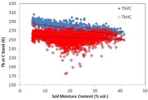
Tbin H polarization appears to be less related to SMC than
V polarization, probably due to the greater influence of the surface features. Figure 3 represents theTbmeasurements in
both H and V polarizations for the entire available dataset. The computed regression equations are
TbV= −76.5SMC+290.31K(R2=0.56) (3a)
TbH= −20.96SMC+259.11K(R2=0.03). (3b)
Additional parameters include:
– The AMSR-ETbat X-band (H and V polarizations) for
computing PIXand correcting for the effect of low
veg-etation on soil emission.
– TheTbat Ka-band, V polarization, used to normalize
for the daily and seasonal variation of the surface tem-perature, due to its strong relationship with the latter pa-rameter (Owe and Van De Griend, 2001; Paloscia et al., 2006).
Fig. 1. Flowchart of the HydroAlgo algorithm for estimating both snow depth (SD) and soil moisture (SMC).
a type of nonlinear, least-mean-square-interpolation formula for the discrete set of data points in the training set. The algo-rithm chosen for the training phase was the back-propagation learning rule, which is an iterative gradient descent algorithm that is designed to minimize the mean square error between the desired target vectors and the actual output vectors. It should be noted that the gradient-descent method sometimes suffers from slow convergence, due to the presence of one or more local minima, which may also affect the final result of the training. In order to overcome this problem, the training was repeated several times, with a resetting of the initial con-ditions and a verification that each training process led to the same convergence results in terms ofR2and RMSE, by in-creasing it until negligible improvements were obtained. This was done in order to define the minimal ANN architecture ca-pable of providing an adequate fit for the training data, so as to prevent overfitting problems. Overfitting is related to the oversizing of the ANN, and may cause considerable errors when testing ANN with input data that is not included in the training set. In order to define the optimal ANN architecture, after the training phase, the ANN was tested using data not included in the training set, and the training and testing re-sults were then compared. The ANN configuration was then increased, until the ANN architecture was found to have a negligible improvement in the training and a worsening in the test results. A configuration with two hidden layers of ten perceptrons each was finally chosen as the optimal one. ANN training and test
The training of the ANN was carried out by using the exten-sive experimental dataset available on the Mongolia and Aus-tralia sites, integrated by model simulations. PIXwas able to
[image:7.595.55.285.62.267.2]Fig. 2. The Plant Water Content (PWC, in kg m−2)estimated from the X-band Polarization index, compared to the PWC estimated from NDVI, for a large area in Africa (0–20◦N/16◦–17◦E). The line represents the regression equation.
Fig. 3. The brightness temperatures (Tb) measured at C-band (in V
and H pol.) in Australian and Mongolian test sites as a function of volumetric SMC (m3m−3).
indicate the vegetation seasonal cycle of the Australian site, as is shown for example for one of the ground stations in the site (ADELONG ROCHEDALE station, Lat. 35.37◦S, Lon. 148.06◦E) (Fig. 4), whereas the semi-arid region of Mongolia did not show any significant periodic variation.
On both these sites, the Tb at C-band, in V polarization
[image:7.595.309.546.355.514.2]Fig. 4. The X-band Polarization Index (PIX) computed for the
ADELONG ROCHEDALE station (Australia, Lat. 35.373◦S, Lon. 148.066◦E) as a function of time.
Fig. 5. PIX, derived from the AMSR-E measurements, as a
func-tion of the optical depth estimated by using the Nelder–Mead inver-sion method. The obtained regresinver-sion is: PIX=11.18 exp (−3.12τ )
(R2=0.99).
correction for vegetation effects through its correlation to the optical depth.
In order to increase the amount of data for the training and testing processes, the experimental dataset described above was enlarged with simulated data by using the Ra-diative Transfer Theory in the formulation of the tau-omega model. Model simulations performed at all the frequen-cies and polarizations considered were iterated by randomly varying the input values of SMC and surface temperature,
Ts, in a reasonable range of expected values (i.e. SMC from
0.05 m3m−3 to 0.5 m3m−3, andT
s from 275 K to 320 K).
The lower threshold of 275 K was selected in order to elim-inate frozen soils. The effect due to surface roughness was taken into account by including in the ANN training setTb
data corresponding to different surface roughness conditions. In the end, a dataset of 10 000 simulated values ofTb was
[image:8.595.51.286.63.213.2]generated. The dielectric constant was derived from the input of SMC by means of the model from Dobson et al. (1985),
Fig. 6. Experimental (red) and simulated (blue)Tbdata (V pol.) of
the whole dataset (Australia and Mongolia) as a function of SMC, in m3m−3(top: C-band; bottom: Ka band).
Table 1. Comparison between measured and estimated averaged values of SMC (in m3m−3) for the Scrivia test area at different dates.
SMC measured SMC estimated
Dates (m3m−3) (m3m−3)
07 November 2003 0.293 0.295
04 June 2004 0.204 0.175
31 March 2008 0.236 0.231
24 April 2008 0.298 0.244
01 July 2008 0.244 0.198
30 September 2008 0.143 0.135
29 May 2009 0.237 0.199
18 June 2009 0.228 0.182
and the range of the other two inputs required by the model, namely the optical depth (τ )and the equivalent single scat-tering albedo (ω), was set so as to assure consistency between the model simulations and the experimental data.
Since no direct measurements of vegetation were included in the dataset, the values of τ andω were estimated from the experimental data by using a direct minimization method. This was done by searching for a couple ofτ andωvalues that would minimize the RMS error between theTb
[image:8.595.50.287.275.425.2] [image:8.595.317.536.440.562.2]Fig. 7. SMC estimated by using the ANN algorithm as a function of SMC measured on ground for the part of Australian and Mongolian dataset not used for training.
The minimization was implemented through the Nelder– Mead simplex algorithm (Nelder and Mead, 1965), which is a popular search method for multidimensional unconstrained minimization.
In this case, the Cost Function (CF) to be minimized by varyingτ andωwas
CF(τ, ω)=sqrth(TbVm(f ))−TbVs(f )2
+(TbHm(f )−TbHs(f ))2
i
(4) where:
– TbVm(f )andTbHm(f )are theTbmeasured at thef
fre-quency (from C- to Ka-band).
– TbVs(f )andTbHs(f )are the outputs of the tau-omega
model for each measured value of SMC and surface temperature, which were obtained by varying theτ and
ωvalues until the minimum of the above function was reached.
The above procedure was repeated for eachTbcouple (V and
H pol.) of the experimental dataset, thus enabling us to as-sociate the estimated values ofτ andωwith each AMSR-E acquisition and to establish empirical relationships between these two quantities and the frequency.
For the dataset considered, theτvalues obtained at C-band ranged between 0.16 and 1.1, while the correspondingω val-ues were between 0.03 and 0.08. The variation ofτ andω
with the frequency was also investigated, in order to estab-lish empirical relationships for deriving their values at fre-quencies higher than C band. For example, the relationships
Table 2. Statistical parameters of the relationships between mea-sured and estimated averaged values of SMC (in m3m−3)for each ARS test area and for both ascending (top) and descending (bottom) orbits.
Ascending Orbits R2 RMSE BIAS Little Washita 0.37 0.046 −0.006 Walnut Gulch 0.30 0.019 −0.0003 Little River 0.28 0.043 0.017
River Creek 0.52 0.039 0.011
Descending Orbits R2 RMSE BIAS Little Washita 0.33 0.048 −0.008 Walnut Gulch 0.26 0.020 0.0011 Little River 0.36 0.039 0.0021
River Creek 0.29 0.065 0.022
between the average values ofτ (f )andω(f )of the entire dataset and the frequency are shown in the following equa-tions
τ (f )=0.0388f+0.08(R2=0.98) (5)
ω(f )=0.0011f+0.0417(R2=0.35) (6) wheref is the frequency in GHz.
The reliability of this inversion method in estimatingτ val-ues was verified by representing the polarization index at X-band (PIX)derived from the AMSR-E as a function ofτ (at the same frequency) estimated as above by using the Nelder– Mead inversion.
The relationship obtained is shown in Fig. 5 and in the following Eq. (7)
PIX=11.18exp(−3.12τ )(R2=0.99) (7)
which is in agreement with the results found in Paloscia and Pampaloni (1988).
Once the relationships (4–7) were assessed, the tau-omega model was iterated 10 000 times with the following random inputs:
– SMC between 0.05 m3m−3and 0.5 m3m−3→
dielec-tric constant→surface reflectivity.
– Surface temperature between 275 K and 320 K.
– τ (C-band) between 0.16 and 1.1,τ at higher frequen-cies computed from Eq. (5).
– ω(C-band) between 0.03 and 0.08,ωat higher frequen-cies computed from the one at C-band.
The results of these iterations, combined with the experi-mental data, are shown in Fig. 6, whereTb at C- (top) and
[image:9.595.332.524.114.248.2]Fig. 8. Temporal trends ofTbat X-, Ku- and Ka- bands and the corresponding snow depth (SD, in cm) measurements obtained for the Siberia
dataset from 2002 to 2009.
Fig. 9. Estimated vs. ground measured SD for the Siberian test area.
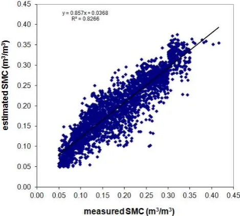
The training of the ANN was carried out by using half (6500) of all these experimental and simulated data. The test performed on the second half of the experimental data pro-duced the diagram of Fig. 7, in which the soil moisture esti-mated by the algorithm (SMCest)is compared with the soil
moisture measured on the ground (SMCmeas). The regression
equation is
SMCest=0.76SMCmeas+4.98 (8)
with a R2=0.8, RMSE=0.035 m3m−3, and BIAS=0.02 m3m−3.
[image:10.595.49.288.290.498.2]This result can be considered to be the main test of the algorithm’s performances in estimating SMC.
Fig. 10. Estimated vs. ground measured SD for the test area in Scan-dinavia (Kautokeino, Sodankyla, Muonio and Pajala stations).
3.2 Estimate of Snow Depth
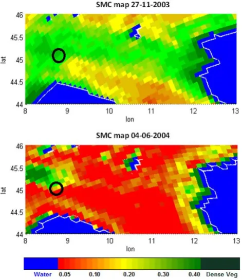
[image:10.595.310.547.291.498.2]Fig. 11. SMC maps generated by using HydroAlgo in North-ern Italy. Maps were carried out on 27 November 2003 and on 4 June 2004. Black circles indicate the ground truth data area.
Since the ANN is not able to separate snow cover from snow-free areas, we used a Frequency Index (FI) as a thresh-old indicator of snow presence, expressed as follows FI= [(TbKuV−TbKaV)+(TbKuH−TbKaH)]/2 (9) where V and H are the polarizations, and Ku and Ka are the frequencies considered.
The analysis of the experimental data collected in the Siberian site and in other regions of the world with SSM/I and AMSR-E (Macelloni et al., 2003) showed that FI is a good indicator of the presence of snow. The threshold for having snow on ground was established in
FI≥4K (10)
Thus, the retrieval of SD was planned in two phases. The first step was the identification of the snow-covered area, by using FI: ANN was then used to retrieve SD.
ANN training and test
In this case, the training of the ANN was carried out by using the extensive experimental dataset available on the Siberian sites. The temporal trends ofTbat X-, Ku- and Ka-band at
V polarization collected from 2002 to 2009 on these sites showed good agreement with the corresponding SD mea-surements for the whole dataset, as can be observed in Fig. 8.
A direct correlation betweenTbat Ka-, X-, and Ku-band and
SD resulted in the following relationships
TbXV= −0.50SD+149.34 (R
2=0.07) (11)
TbKuV= −0.44SD+256.55 (R
2=0.35) (12)
TbKaV= −1.44SD+255.86 (R
2=0.69) (13)
where V is the polarization and Ku (or Ka or X) is the fre-quency band considered.
No model simulations were added to the training of the ANN, due to the very large extent of the database. The training of the ANN was carried out by using half of all these experimental data. The test performed on the second half of the dataset produced the diagram in Fig. 9, in which the SD estimated by the algorithm (SDest)is compared with the SD
measured on the ground (SDmeas). The regression equation
is
SDest=0.78SDmeas+5.97 (14)
with aR2=0.79, RMSE=5.54 cm, and BIAS=0.059 cm. Also in this case, the result can be considered to be the main test for the performances of the algorithm in estimating SD.
4 Validation
Validation of the algorithm was carried out on some test ar-eas in Europe and the US, where ground mar-easurements were available. One area was located in Northern Italy (approx-imately 100×100 km2)and four others of smaller dimen-sions in the US, for SMC. Moreover, a further area in Scan-dinavia (200×100 200 km2)was chosen for SD validation. This validation procedure was also useful in evaluating the performance of HydroAlgo at different spatial scales. 4.1 Soil moisture
The validation of HydroAlgo for the retrieval of SMC was performed on the Scrivia watershed in Italy, where a long-term experimental study devoted to SMC and vegetation was carried out in the hopes of fine-tuning operational procedures for flood forecasting and alert. The validation was repeated for all the dates for which ground measure-ments were available. The results are shown in Table 1. The statistical parameters of the regression between estimated and measured SMC are:R2=0.82, RMSE=0.035 m3m−3,
BIAS=0.09 m3m−3.
A further and more performing test was carried out by comparing AMSR-E data to the ground SMC data collected in four experimental watersheds of the Agricultural Research Service (ARS) in the US, kindly provided by Dr. Tom Jack-son (JackJack-son et al., 2010).
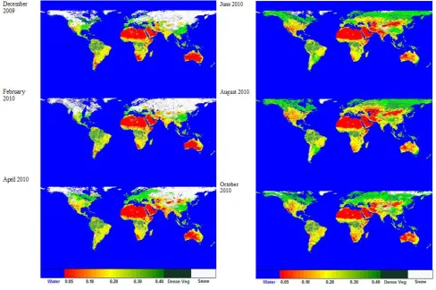
Fig. 12. (a) SMC maps (in m3m−3)of the entire world obtained in December 2009, February and April 2010, by using HydroAlgo. Some AMSR-E scans are missing, as we can see in Africa and North America in February 2010. (b) SMC maps (in m3m−3)of the entire world obtained in June, August, and October 2010, by using HydroAlgo. Some AMSR-E scans are missing, as we can see in Africa and South America (black lines).
These statistical parameters were obtained for each test area and for both ascending and descending orbits.R2is gener-ally not very high, whereas RMSE and BIAS are rather low and≤0.05 m3m3and≤0.02 m3m−3, respectively. Results demonstrated that the algorithm performs within a specified accuracy of≤0.06 m3m−3(Paloscia et al., 2012).
4.2 Snow Depth
The SD retrieval was validated over a test area in Scandi-navia, by comparing the algorithm outputs with the averaged SD measurements of four meteorological stations located in Kautokeino, Sodankyla, Muonio, and Pajala. Once the snow-covered areas had been identified by means of the FI≥4 K threshold, the relationship obtained by comparing the mea-sured on ground SD (SDmeas)and the corresponding outputs
of ANN (SDest)was the following:
SDest=0.81SDmeas+7.54 (15)
with aR2=0.79, RMSE=9.13 cm, and BIAS= −0.95 cm. The results obtained are shown in Fig. 10.
5 Algorithm applications
Once the algorithm was validated on relatively small areas, an attempt to test its validity further on a larger scale was car-ried out. Although it cannot be considered a real validation, due to the absence of corresponding and adequate ground data, this study can be useful for understanding the capability of the algorithm to reasonably estimate SMC, SD and PWC in other regions with respect to those where it has been tested and therefore to also verify its flexibility. This is particularly important for evaluating the capabilities of ANN to general-ize the training phase that was based on data derived from small areas. Although it is difficult to obtain ground data of SMC, SD and PWC in order to validate the algorithm at a so large scale, we have observed that the range of these parame-ters is generally compatible with the climatic regions and the meteorological conditions related to latitude and seasons.
[image:12.595.53.542.63.387.2]Fig. 13. SD maps (in cm) retrieved on Europe before and after heavy snowfall events in December 2009 and 2010. On 15 December 2009 and 9 December 2010 the snow cover is sparse and almost limited to Scandinavia and Alps, whereas, after the events, the snow cover appears to be much more spread and evident even in Central Italy, where the snow depth measured on 20 December 2009 in the area close to Florence (white circle) was about 10 cm on the ground, which is the value estimated by the algorithm.
available, and an evaluation of the resulting maps was thus performed on the basis of climatic and meteorological char-acteristics of the regions of the globe investigated.
5.1 Soil moisture
SMC maps produced with the algorithm over all of Northern Italy are shown in Fig. 11. The maps refer to 27 Novem-ber 2003, and 4 June 2004. In spite of the coarse ground res-olution, a marked difference in SMC between the two dates is
Fig. 14. SD map (in cm) of the entire world obtained by HydroAlgo in December 2009 and February 2010. The greater snow cover in Europe in February is evident. Some AMSR-E scans are missing, as we can see in Africa and North America in February 2010.
SMC maps of the entire world obtained at different dates (December 2009, February, April, August and October 2010) are shown in Fig. 12a, b. Snow cover and forests are masked in the images. At least 4 levels of SMC can easily be iden-tified. Although no ancillary information is available, the re-sults are in reasonable agreement with the climatic and sea-sonal meteorological conditions of the various zones. The slightly higher SMC values for the Arabian and Australian coasts correspond to the presence of sparse vegetation, as these regions are more humid than the desert zones. The seasonal variation in SMC shows an opposite trend in the two hemispheres: e.g. Australia is wetter in August than in February.
5.2 Snow Depth
[image:14.595.309.547.61.422.2]The SD maps of all of Europe, generated in December 2009 and 2010 are shown in Fig. 13, in order to include the Alps, the Apennines, and the Balkan Mountains as well. The snow-covered areas are clearly visible, and at least 4 ranges of SD can also be distinguished. The maps were made before and immediately after heavy snowfall events. On 15 Decem-ber 2009 and 9 DecemDecem-ber 2010, the snow cover was sparse and almost limited to Scandinavia and the Alps, whereas the snow cover after the events appears to have been much more spread and evident even in Central Italy, where the SD mea-sured on the ground in the area close to Florence was about 10 cm, which is the value estimated by the algorithm.
Fig. 15. Vegetation maps of PWC for the entirety of Africa extracted from PIX(top) and NDVI (bottom), respectively. The relationship
between NDVI and PWC was derived from Jackson et al. (2004).
Lastly, two SD maps of the whole world, obtained in De-cember 2009 and February 2010 by using HydroAlgo, are shown in Fig. 14. The presence of snow, especially in the Northern hemisphere, is clearly pointed out.
5.3 Vegetation biomass
In this context, vegetation maps of PWC (kg m−2)are gener-ated from PIXmainly to mask dense vegetation in SMC and
SD maps and to correct the SMC estimate for the effects of low vegetation. However, these maps can represent an addi-tional output of the algorithm.
For example, a vegetation map of Africa computed from PIX is shown in Fig. 15a and b, in which the PWC
ob-tained from PIX is compared with the one derived from
(optical) NDVI obtained from Free Vegetation Products (http://free.vgt.vito.be/home.php). The direct comparison in the two maps between the PWC values from SPOT4 and from PIX, carried out pixel by pixel gave the
and BIAS=1.89×10⁻²kg m−2. According to these results,
the vegetation maps on a global scale can reasonably be generated by using PIX as a byproduct of the HydroAlgo,
instead of NDVI, in view of the advantage of using the same sensor for all applications.
6 Summary and conclusions
A new algorithm (HydroAlgo) for generating simulta-neous maps of SMC and SD from AMSR-E data has been implemented within the framework of the GCOM-W/AMSR-2 project of JAXA and the Italian National Project ASI/PROSA, for the purpose of developing products useful for hydrological applications and natural disasters manage-ment. The algorithm makes exclusive use of AMSR-E-like data. C-band channel provides basic information for the re-trieval of SMC, while SD is essentially obtained from X-, Ku- and Ka-band channels. Additional information on sur-face temperature and vegetation cover, which was useful for improving the retrieval accuracy of the algorithm, was ob-tained from theTbat Ka-band (V polarization) and from the
Polarization Index at X band (PIX), respectively. The latter
quantity made possible the generation of maps of vegetation biomass (VB, expressed as PWC) as an auxiliary product. No other ancillary data were required to obtain the results presented here.
HydroAlgo was able to separate 4–5 levels of SMC and SD at a nominal ground resolution of 10 km×10 km, by us-ing a specific algorithm for improvus-ing the spatial resolution. Both SMC and SD were retrieved by using ANN methods trained with a large set of experimental data. For the retrieval of SMC, the dataset was enriched by model simulations. The global maps of SMC, SD and PWC were reprojected over a fixed grid, in geographical coordinates with a spatial resolu-tion of about 10 km×10 km. This represented an improve-ment in the spatial resolution of the input C- and X-band channels involved in SMC and PWC estimates. Processing an entire day of AMSR-E acquisitions required about 20 min. In order to compute a reliability index of the output prod-ucts, the entire process took into account the percentage of bad input data (including those affected by RFI) and the esti-mate of output parameters outside the established range. This index has been listed in the header file associated with each output.
Furthermore, the algorithm was applied at several spatial scales over different regions of the Earth. Although this part of the paper cannot be considered a real validation, due to the absence of adequate ground data, it is important to note that the algorithm is able to reasonably follow the variations of SMC and SD at different latitudes and in various climatic conditions. In any case, additional tests on different areas and seasons would be desirable, in order to evaluate more thor-oughly the operational capabilities of the implemented code.
Acknowledgements. This research work was partially supported by
the ASI/PROSA Italian project, the JAXA ADEOS-II/AMSR-E and GCOM/AMSR2 missions, and by the CTOTUS project, which was co-funded by Regione Toscana within the framework of the “Pro-gramma Operativo Regionale – obiettivo Competitivit`a Regionale e Occupazione” – POR-CReO FESR 2007-2013.
The authors wish to thank JAXA for providing the Mongolian Plateau, Australian and Siberian ground datasets. In particular, we would like to thank Ichirow Kaihotsu, Toshio Koike, and Keiji Imaoka for their kind help and support. Furthermore, the authors would like to express their gratitude to Tom Jackson for kindly making available the archive of USDA/ARS data for a more accurate validation of the soil moisture algorithm.
Edited by: J. Liu
References
Angiuli, E., Del Frate, F., and Monerris, A.: Application of Neural Networks to Soil Moisture Retrievals from L-Band Radiometric Data, Proc. IEEE Intern. Geosci Remote Sens. Symp., IGARSS 2008, Boston, MA, USA, II-61–II-64, 2008.
Balling, J., Søbjoerg, S., Kristensen, S., and Skou, N.: RFI and SMOS: Preparatory campaigns and first observations from space, Proc. 11th Specialist Meeting on Microwave Radiometry and Re-mote Sensing of the Environment (MicroRad), Washington, DC, March 2010, 282–287, 2010.
Barre, H. M. J., Duesmann, B., and Kerr, Y. H.: SMOS: The Mission and the System, IEEE T. Geosci. Remote Sens., 46, 587–593, March, 2008.
Bates, B. C., Kundzewicz, Z. W., Wu, S., and Palutikof, J. P. (Eds.): IPCC Secretariat, Geneva, 210 pp., June, 2008.
Becker, F. and Choudhury, B.: Relative Sensitivity of Normalized Difference Vegetation Index (NDVI) and Microwave Polariza-tion Difference Index (MPDI) for VegetaPolariza-tion and DesertificaPolariza-tion Monitoring, Remote Sens. Environ., 24, 297–311, 1988. Borodin, L., Kirdjashev, K., Stakankin, J., and Chuklantsev, A.:
Mi-crowave radiometry of forest fires, Radiotekhnika Electronica, 21, p. 1945, 1976.
Calvet, J.-C., Wigneron, J.-P., Mougin, E., Kerr, Y., and Brito, J.: Plant water content and temperature of the Amazon forest from satellite microwave radiometry, IEEE T. Geosci. Remote Sens., 32, 397–408, 1994.
Chai, S.-S., Walker, J. P., Makarynskyy, O., Kuhn, M., Veenendaal, B., and West, G.: Use of Soil Moisture Variability in Artificial Neural Network Retrieval of Soil Moisture, Remote Sens., 2, 166–190, 2010.
Chang A. T. C., Foster, J. L., Hall, D. K., Rango, A., and Hartline, B. K.: Snow water equivalent estimation by microwave radiometry, Cold Reg. Sci. Technol., 5, 259–267, 1982.
Chang, A. T. C., Foster, J. L., and Hall, D. K.: Nimbus-7 derived global snow cover parameters, Ann. Glaciol., 9, 39–44, 1987. Choudhury, B. J.: Monitoring global land surface using Nimbus-7
Davenport, I. J., Fern´andez-G´alvez, J., and Gurney, R. J.: A Sensi-tivity Analysis of Soil Moisture Retrieval From the Tau–Omega Microwave Emission Model, IEEE T. Geosci. Remote Sens., 43, 1304–1316, June, 2005.
Davis, D. T., Chen, Z., Tsang, L., Hwang, J. -N., and Chang, A. T. C.: Retrieval of snow parameters by iterative inversion of a neural network, IEEE T. Geosci. Remote Sens., 31, 842–851, 1993. Del Frate, F., Ferrazzoli, P., and Schiavon, G.: Retrieving soil
mois-ture and agricultural variables by microwave radiometry using neural networks, Remote Sens. Environ, 84, 174–183, 2003. Dobson, M. C., Ulaby, F. T., Hallikainen, M. T., and El-Rayes, M.
A.: Microwave dielectric behavior of wet soil – Part II: Dielectric mixing models, IEEE T. Geosci. Remote Sens., GE-23, 35–46, January, 1985.
Entekhabi, D., Njoku, E. G., O’Neill, P. E., Kellogg, K. H., Crow, W. T., Edelstein, W. N., Entin, J. K., Goodman, S. D., Jackson, T. J., Johnson, J., Kimball, J., Piepmeier, J. R., Koster, R. D., Mar-tin, N., McDonald, K. C., Moghaddam, M., Moran, S., Reichle, R., Shi, J. C., Spencer, M. W., Thurman, S. W., Tsang, L., and Van Zyl, J.: The Soil Moisture Active Passive (SMAP) Mission, P. IEEE, 98, 704–716, 2010.
Goodison, B. and Walker, A.: Canadian development and use of snow cover information from passive microwave satellite data, in: Passive Microwave Remote Sensing of Land-Atmosphere In-teractions, edited by: Choudhury, B., Kerr, Y., Njoku, E., and Pampaloni, P., Utrecht, The Netherlands, VSP BV, 245–62, 1995. Grody, N. C. and Basist, A. N.: Global Identification of snow cover using SSM/I measurements, IEEE T. Geosci. Remote Sens., 34, 237–249, 1996.
Hall, D. K., Foster, J. L., Salomonson, V. V., Klein, A. G., and Chien, J. Y. L.: Development of a technique to assess snow-cover mapping errors from space, IEEE T. Geosci. Remote Sens., 39, 432–438, February, 2001.
Hallikainen, M. T. and Jolma, P. A.: Comparison of algorithms for retrieval of snow water equivalent from NIMBUS-7 SMMR data I Finland, IEEE T. Geosci. Remote Sens., 30, 124–131, January, 1992.
Hallikainen, M. T., Jolma, P. A., and Hyyppa, J. M.: Satellite Mi-crowave Radiometry of Forest and Surface Types in Finland, IEEE T. Geosci. Remote Sens., 26, 622–628, 1988.
Hofer, R. and M¨atzler, C.: Investigation of snow parameters by ra-diometry in the 3- to 60-mm wavelength region, J. Geophys. Res., 85, 453–460, 1980.
Hornik, K.: Multilayer feed forward networks are universal approx-imators, Neural Netw., 2, 359–366, 1989.
Jackson, T. J.: Measuring surface soil moisture using passive mi-crowave remote sensing, Hydrol. Process., 7, 139–152, 1993. Jackson, T. J. and Hsu, A. Y.: Soil moisture and TRMM microwave
imager relationships in the Southern Great Plains 1999 (SGP99) Experiment, IEEE T. Geosci. Remote Sens., 39, 1632–1642, Au-gust, 2001.
Jackson, T. J., Schmugge, T., and Wang, J.: Passive microwave re-mote sensing of soil moisture under vegetation canopies, Water Resour. Res., 18, 1137–1142, 1982.
Jackson, T. J., Gasiewski, A. J., Oldak, A., Klein, M., Njoku, E. G., Yevgrafov, A., Christiani, S., and Bindlish, R.: Soil moisture retrieval using the C-band polarimetric scanning radiometer dur-ing the Southern Great Plains 1999 Experiment, IEEE T. Geosci. Remote Sens., 40, 2151–2161, October, 2002.
Jackson, T. J., Chen, D., Cosh, M., Li, F., Anderson, M., Walthall, C., Doriaswamy, P., and Hunt, E. R.: Vegetation water content mapping using Landsat data derived normalized difference water index for corn and soybeans, Remote Sens. Environ., 92, 475– 482, 2004.
Jackson, T. J., Cosh, M. H., Bindlish, R., Starks, P. J., Bosch, D. D., Seyfried, M., Goodrich, D. C., Moran, M. S., and Jinyang, D.: Validation of Advanced Microwave Scanning Radiometer Soil Moisture Products, IEEE T. Geosci. Remote Sens., 48, 4256– 4272, 2010.
Jiang, H. and Cotton, W. R.: Soil moisture estimation using an ar-tificial neural network: a feasibility study, Can. J. Remote Sens., 30, 827–839, 2004.
Jin, Y. Q.: Snow depth inverted by scattering indices of SSM/I chan-nels in a mesh graph, Int. J. Remote Sens., 18, 1843–1849, 1997. Kawanishi, T., Sezai, T., Ito, Y., Imaoka, K., Takeshima, T., Ishido, Y., Shibata, A., Miura, M., Inahata, H., and Spencer, R. W.: The Advanced Microwave Scanning Radiometer for the Earth Ob-serving System (AMSR-E), NASDA’s contribution to the EOS for global energy and water cycle studies, IEEE T. Geosci. Re-mote Sens., 41, 184–194, February, 2003.
Kelly, R. E., Chang, A. T., Tsang, L., and Foster, J. L.: A prototype AMSR-E global snow area and snow depth algorithm, IEEE T. Geosci. Remote Sens., 41, 230–242, February, 2003.
Kerr, Y. H., Waldteufel, P., Wigneron, J.-P., Delwart, S., Cabot, F., Boutin, J., Escorihuela, M.-J., Font, J., Reul, N., Gruhier, C., Ju-glea, S. E., Drinkwater, M. R., Hahne, A., Martin-Neira, M., and Mecklenburg, S.: The SMOS Mission: New Tool for Monitor-ing Key Elements of the Global Water Cycle, IEEE Proc., 98, 666–687, 2010.
Kruopis, N., Praks, J., Arslan, A. N., Alasalmi, H., Koskinen, M. J., and Hallikainen, M. T.: Passive Microwave Measurements of Snow-Covered Forest Areas in EMAC’95 , IEEE T. Geosci. Re-mote Sens., 37, 2699–2705, 1999.
Kurvonen, L., Pulliainen, J., and Hallikainen, M. T.: Monitoring of Boreal Forests with Multitemporal Special Sensor Microwave Imager, Radio Sci., 33, 731–744, 1998.
Linden, A. and Kinderman, J.: Inversion of multilayer nets, in: Proc. Int. Joint Conf. Neural Netw., II, 425–430, 1989.
Liou, Y.-A., Shou-Fang, L., and Wen-June, W.: Retrieving Soil Moisture from Simulated Brightness Temperatures by a Neural Network, IEEE T. Geosci. Remote Sens., 39, 1662–1672, 2001. Liu, J. and Yang, H.: Spatially explicit assessment of global
con-sumptive water uses in cropland: green and blue water, J. Hy-drol., 384, 187–197, doi:10.1016/j.jhydrol.2009.11.024, 2010. Liu, J. G.: Smoothing Filter Based Intensity Modulation: a Spectral
Preserve Image Fusion Technique for Improving Spatial Details, Int. J. Remote Sens., 21, 3461–3472, 2000.
Liu, J. G., Zehnder, A. J. B., and Yang, H.: Global consump-tive water use for crop production: The importance of green water and virtual water, Water Resour. Res., 45, W05428, doi:10.1029/2007WR006051, 2009.
Liu, S.-F., Liou, Y.-A., Wang, W.-J., Wigneron, J.-P., and Jann-Bin, L.: Retrieval of Crop Biomass and Soil Moisture from Measured 1.4 and 10.65 Ghz Brightness Temperatures, IEEE T. Geosci. Re-mote Sens., 40, 1260–1268, 2002.
Mo, T., Choudhury, B. J., Schmugge, T. J., Wang, J. R., and Jackson, T. J.: A model for microwave emission from vegetation covered fields, J. Geophys. Res., 87, 11229–11237, 1982.
Nelder, J. A. and Mead, R.: A Simplex Method for Function Mini-mization, Comput. J., 7, 308–313, 1965.
Njoku, E. G.: Updated daily AMSR-E/Aqua Daily L3 Surface Soil Moisture, Interpretive Parameters, & QC EASE-Grids V06, from July to August 2003, Boulder, Colorado USA, National Snow and Ice Data Center, Digital media, 2003.
Njoku, E. G. and Kong, J. A.: Theory for Passive Microwave Re-mote Sensing of Near-Surface Soil Moisture, J. Geophys. Res., 82, 3108–3118, 1977
Njoku, E. G. and Li, L.: Retrieval of Land Surface Parameters Using Passive Microwave Measurements at 6–18 GHz, IEEE T. Geosci. Remote Sens., GE-37, 79–93, 1999.
Njoku, E. G., Koike, T., Jackson, T., and Paloscia, S.: Retrieval of soil moisture from AMSR data, in: Microwave Radiometry for Remote Sensing of the Earth’s Surface and Atmosphere, edited by: Pampaloni, P. and Paloscia, S., Utrecht, The Netherlands: VSP press, 525–533, 2000.
Njoku, E. G., Jackson, T. J., Lakshmi, V., Chan, T. K., and Nghiem, S. V.: Soil Moisture Retrieval from AMSR-E, IEEE T. Geosci. Remote Sens., 41, 215–229, February, 2003.
Njoku, E. G., Aschroft, P., Chan, T. K., and Li, L.: Global Survey and Statistics of Radio-Frequency Interference in AMSR-E Land Observations, IEEE T. Geosci. Remote Sens., 43, 938–947, May, 2005.
Owe, M. and Van De Griend, A. A.: “On the relationship be-tween thermodynamic surface temperature and high-frequency (37 GHz) vertically polarized brightness temperature under semi-arid conditions”, Int. J. Remote Sens., 22, 3521–3532, Novem-ber, 2001.
Owe, M., de Jeu, R., and Walker, J.: A methodology for surface soil moisture and vegetation optical depth retrieval using the mi-crowave polarization difference index, IEEE T. Geosci. Remote Sens., 39, 1643–1654, August, 2001.
Owe, M., de Jeu, R., and Holmes, T.: Multisensor historical clima-tology of satellite-derived global land surface moisture, J. Geo-phys. Res., 113, F01002, doi:10.1029/2007JF000769, 2008. Paloscia, S.: Microwave emission from vegetation, in: Passive
Microwave Remote Sensing of Land-Atmosphere Interactions, edited by: Choudhury, B., Kerr, Y., Njoku, E., and Pampaloni, P., Utrecht, The Netherlands: VSP BV, 357–374, 1995.
Paloscia, S. and Pampaloni, P.: Microwave Polarization Index for Monitoring Vegetation Growth, IEEE T. Geosci. Remote Sens., GE-26, 617–621, September, 1988.
Paloscia, S. and Pampaloni, P.: Microwave vegetation indexes for detecting biomass and water conditions of agricultural crops, Re-mote Sens. Environ., 40, 15–26, 1992.
Paloscia, S., Pampaloni, P., Chiarantini, L., Coppo P., Gagliani, S., and Luzi, G.: Multifrequency passive microwave remote sensing of soil moisture and roughness, Int. J. Remote Sens., 14, 467– 484, 1993.
Paloscia, S., Macelloni, G., Santi, E., and Koike, T.: A multifre-quency algorithm for the retrieval of soil moisture on a large scale using microwave data from SMMR and SSM/I satellites, IEEE T. Geosci. Remote Sens., 39, 1655–1661, August, 2001. Paloscia, S., Macelloni, G., and Santi, E.: Soil Moisture
Esti-mates from AMSR-E Brightness Temperatures by using a
Dual-Frequency Algorithm, IEEE T. Geosci. Remote Sens., 44, 3135– 3144, November, 2006.
Paloscia, S., Pettinato, S., Santi, E., Pierdicca, N., Pulvirenti, L., No-tarnicola, C., Pace, G., and Reppucci, A.: “Soil moisture mapping using Sentinel-1 images: The proposed approach and its prelim-inary validation carried out in view of an operational product”, Proc. of SPIE Remote Sensing conference 8179 on SAR Image Analysis, Modeling, and Techniques XI, Prague, 817904, 21–22 September, 2011.
Paloscia, S., Santi, E., Pettinato, S., Mladenova, I., Jackson, T., and Bindlish, R.: A comparison between two algorithms for the re-trieval of soil moisture on a regional scale by using AMSR-E data, IEEE T. Geosci. Remote Sens., Special Issue of MicroRad, submitted, 2012.
Pampaloni, P.: Microwave Radiometry of Forests, Waves Random Media, 14, S275–S298, 2004.
Pettinato, S., Brogioni, M., Santi, E., Paloscia, S., and Pampaloni, P.: An Operational Algorithm for Snow Cover Mapping in Hy-drological Applications, IEEE International Geoscience and Re-mote Sensing Symposium, IGARSS 2009, IV, 964–967, July, 2009.
Pulliainen, J. T.: Mapping of snow water equivalent and snow depth in boreal and sub-arctic zones by assimilating space-borne mi-crowave radiometer data and ground-based observations, Remote Sens. Environ., 101, 257–269, 2006.
Pulliainen, J. T. and Hallikainen, M.: Retrieval of regional snow wa-ter equivalent from space-borne passive microwave observations, Remote Sens. Environ., 75, 76–85, 2001.
Pulliainen, J. T., Grandell, J., and Hallikainen, M. T.: HUT snow emission model and its applicability to snow water equivalent retrieval, IEEE T. Geosci. Remote Sens., 37, 1378–1390, 1999. Rott, H. and Nagler, T.: Intercomparison of snow retrieval
algo-rithms by means of spaceborne microwave radiometry, in: Pas-sive Microwave Remote Sensing of Land-Atmosphere Interac-tions, edited by: Choudhury, B., Kerr, Y., Njoku, E., and Pam-paloni, P., Utrecht, The Netherlands: VSP BV, 239–243, 1995. Santi, E.: An application of SFIM technique to enhance the spatial
resolution of microwave radiometers, Int. J. Remote Sens., 31, 2419–2428, 2010.
Santi, E., Pettinato, S., Paloscia, S., and Pampaloni, P.: Ground-Based Microwave Investigations of Forest Plots in Italy, IEEE T. Geosci. Remote Sens., 47/9, 3016–3025, 2009.
Schwank, M., V¨olksch, I., Wigneron, J. P., Kerr, Y. H., Mialon, A., de Rosnay, P., and M¨atzler, C.: Comparison of Two Bare-Soil Reflectivity Models and Validation With L-Band Radiometer Measurements, IEEE T. Geosci. Remote Sens., 48, 325–337, 2010.
Shibata, A., Imaoka, K., and Koike, T., AMSR/AMSR-E Level 2 and 3 Algorithm Developments and Data Validation Plans of NASDA, IEEE T. Geosci. Remote Sens., 41, 195–203, February, 2003.
Shimoda, H.: Global change observation mission, IEEE Interna-tional Geoscience and Remote Sensing Symposium, IGARSS 2009, 5, 228–231, July, 2009.
Shutko, A. M.: Microwave radiometry of lands under natural and artificial moistening, IEEE T. Geosci. Remote Sens., GE-20, 18– 26, 1982.
in Preparation for SMOS, IEEE T. Geosci. Remote Sens., 48, 1398–1407, March, 2010.
Tedesco, M., Pulliainen, J., Takala, M., Hallikainen, M., and Pam-paloni, P.: Artificial Neural Network Based Techniques for the Retrieval of SWE And Snow Depth From SSM/I Data, Remote Sens. Environ., 90, 76–85, 2004.
Tsang, L. and Jackson, T. (Eds): IEEE Proceedings Special Issue on Satellite Remote Sensing, 98, May, 2010.
Tsang, L., Chen, Z., Oh, S., Marks, R. J., and Chang, A. T. C.: Inver-sion of snow parameters from passive remote sensing microwave measurements by a neural network trained with a multiple scat-tering model, IEEE T. Geosci. Remote Sens., 30, 1015–1024, 1992.
Tsang, L., Chen, C., Chang, A. T. C., Guo, J., and Ding, K.: Dense media radiative transfer theory based on quasicrystalline approx-imation with applications to passive microwave remote sensing of snow, Radio Sci., 35, 731–749, 2000.
Ulaby, F. T. and Stiles, W. H.: The active and passive microwave response to snow parameters, 2: Water equivalent, J. Geophys. Res., 85, 10457–1049, 1980.
Vinnikov, K., Robock, A., Qiu, S., Entin, J., Owe, M., Choudhury, B., Hollinger, S., and Njoku, E.: Satellite remote sensing of soil moisture in Illinois, USA, J. Geophys. Res., 104, 4145–4168, 1999.
Wagner, W., Naeimi, V., Scipal, K., de Jeu, R., and Mart´ınez-Fern´andez, J.: Soil moisture from operational meteorological satellites, Hydrogeol. J., 15 121–131, 2007a.
Wagner, W., Bl¨oschl, G., Pampaloni, P., Calvet, J.-C., Bizzarri, B., Wigneron, J.-P., and Kerr, Y.: Operational readiness of mi-crowave remote sensing of soil moisture for hydrologic applica-tions, Nord. Hydrol., 38, 1–20, IWA Publishing, 2007b. Wang, J. R. and Choudhury, B. J.: Remote sensing of soil moisture
content over bare field at 1.4 GHz frequency, J. Geophys. Res., 86, 5277–5282, 1981.
Wang, J. R. and Choudhury, B. J.: Passive microwave radiation from soil: Examples of emission models and observations, in: Passive Microwave Remote Sensing of Land–Atmosphere Interactions, edited by: Choudhury, B., Kerr, Y., Njoku, E., and Pampaloni, P., Utrecht, The Netherlands: VSP, 1995.
Wigneron, J.-P., Chanzy, A., Calvet, J.-C., and Bruguier, N.: A sim-ple algorithm to retrieve soil moisture and vegetation biomass using passive microwave measurements over crop fields, Remote Sens. Environ., 51, 331–341, 1995.
Wigneron, J.-P., Calvet, J.-C., Pellarin, T., Van de Griend, A. A., Berger, M., and Ferrazzoli, P.: Retrieving near-surface soil mois-ture from microwave radiometric observations: current status and future plans, Remote Sens. Environ., 85, 489–506, 2003. Zang, C. F., Liu, J., van der Velde, M., and Kraxner, F.: Assessment