Exploring the impact of forcing error characteristics on physically based snow simulations within a global sensitivity analysis framework

www.hydrol-earth-syst-sci.net/19/3153/2015/ doi:10.5194/hess-19-3153-2015

© Author(s) 2015. CC Attribution 3.0 License.

Exploring the impact of forcing error characteristics

on physically based snow simulations within a global

sensitivity analysis framework

M. S. Raleigh1, J. D. Lundquist2, and M. P. Clark1

1_{National Center for Atmospheric Research, Boulder, Colorado, USA}

2_{Civil and Environmental Engineering, University of Washington, Seattle, Washington, USA}

Correspondence to: M. S. Raleigh ([email protected])

Received: 24 October 2014 – Published in Hydrol. Earth Syst. Sci. Discuss.: 16 December 2014 Revised: 17 June 2015 – Accepted: 18 June 2015 – Published: 20 July 2015

Abstract. Physically based models provide insights into key hydrologic processes but are associated with uncertainties due to deficiencies in forcing data, model parameters, and model structure. Forcing uncertainty is enhanced in snow-affected catchments, where weather stations are scarce and prone to measurement errors, and meteorological variables exhibit high variability. Hence, there is limited understanding of how forcing error characteristics affect simulations of cold region hydrology and which error characteristics are most important. Here we employ global sensitivity analysis to ex-plore how (1) different error types (i.e., bias, random errors), (2) different error probability distributions, and (3) different error magnitudes influence physically based simulations of four snow variables (snow water equivalent, ablation rates, snow disappearance, and sublimation). We use the Sobol’ global sensitivity analysis, which is typically used for model parameters but adapted here for testing model sensitivity to coexisting errors in all forcings. We quantify the Utah Energy Balance model’s sensitivity to forcing errors with 1 840 000 Monte Carlo simulations across four sites and five different scenarios. Model outputs were (1) consistently more sensi-tive to forcing biases than random errors, (2) generally less sensitive to forcing error distributions, and (3) critically sen-sitive to different forcings depending on the relative magni-tude of errors. For typical error magnimagni-tudes found in areas with drifting snow, precipitation bias was the most important factor for snow water equivalent, ablation rates, and snow disappearance timing, but other forcings had a more dom-inant impact when precipitation uncertainty was due solely to gauge undercatch. Additionally, the relative importance of

forcing errors depended on the model output of interest. Sen-sitivity analysis can reveal which forcing error characteristics matter most for hydrologic modeling.

1 Introduction

There are fewer detailed studies focusing on forcing un-certainty relative to the number of parametric and structural uncertainty studies (Bastola et al., 2011; Benke et al., 2008; Beven and Binley, 1992; Butts et al., 2004; Clark et al., 2008, 2011b, 2015a, b; Essery et al., 2013; Georgakakos et al., 2004; Jackson et al., 2003; Kelleher et al., 2015; Kuczera and Parent, 1998; Liu and Gupta, 2007; Refsgaard et al., 2006; Slater et al., 2001; Smith et al., 2008; Vrugt et al., 2003a, b, 2005; Yilmaz et al., 2008). Di Baldassarre and Montanari (2009) suggest that forcing uncertainty has attracted less at-tention because it is “often considered negligible” relative to parametric and structural uncertainties. Nevertheless, forcing uncertainty merits more attention in some cases, such as in snow-affected watersheds where meteorological and energy balance measurements are scarce (Bales et al., 2006; Raleigh, 2013; Schmucki et al., 2014) and prone to errors due to en-vironmental or instrumental factors (Huwald et al., 2009; Lundquist et al., 2015; Rasmussen et al., 2012). Forcing un-certainty is enhanced in complex terrain where meteorologi-cal variables exhibit high spatial variability (Feld et al., 2013; Flint and Childs, 1987; Herrero and Polo, 2012; Lundquist and Cayan, 2007). As a result, the choice of forcing data can yield substantial differences in calibrated model parameters (Elsner et al., 2014) and in modeled hydrologic processes, such as snowmelt and evapotranspiration (Mizukami et al., 2014; Wayand et al., 2013). Thus, forcing uncertainty de-mands more attention in snow-affected watersheds.

Previous work on forcing uncertainty in snow-affected re-gions has yielded basic insights into how forcing errors prop-agate to model outputs and which forcings introduce the most uncertainty in specific outputs. However, these studies have typically been limited to (1) empirical/conceptual models (He et al., 2011a, b; Raleigh and Lundquist, 2012; Shamir and Georgakakos, 2006; Slater and Clark, 2006), (2) errors for a subset of forcings (e.g., precipitation or temperature only) (Burles and Boon, 2011; Dadic et al., 2013; Durand and Margulis, 2008; Lapo et al., 2015; Xia et al., 2005), (3) model sensitivity to choice of forcing parameterization (e.g., long-wave) without considering uncertainty in parameterization inputs (e.g., temperature and humidity) (Guan et al., 2013), and (4) simple representations of forcing errors (e.g., Kavet-ski et al., 2006a, b). The last is evident in studies that only consider single types of forcing errors (e.g., bias) and sin-gle distributions (e.g., uniform) and examines errors sepa-rately (Burles and Boon, 2011; Koivusalo and Heikinheimo, 1999; Raleigh and Lundquist, 2012; Xia et al., 2005). Lapo et al. (2015) show that biases have a greater impact than random errors on modeled snow water equivalent and sur-face temperature but their analysis only considers longwave and shortwave forcings and considers errors separately. Ex-amining uncertainty in one factor at a time remains popu-lar but fails to explore the uncertainty space adequately, ig-noring potential interactions between forcing errors (Saltelli and Annoni, 2010; Saltelli, 1999). In contrast, global sensi-tivity analysis explores the uncertainty space more

compre-hensively by considering uncertainty in multiple factors at the same time.

The purpose of this paper is to use global sensitivity anal-ysis to assess how specific forcing error characteristics in-fluence outputs of a physically based snow model. To our knowledge, no previously published study has investigated this topic in snow-affected regions. It is unclear how (1) dif-ferent error types (bias vs. random errors), (2) difdif-ferent er-ror distributions, and (3) different erer-ror magnitudes across all forcings affect model output. The impact of forcing errors on models can be tested by corrupting forcings with specified characteristics (e.g., artificial biases and random errors) and quantifying the impact on model outputs (e.g., Oudin et al., 2006; Spank et al., 2013), but we are unaware of any de-tailed studies that have done this type of experiment for all meteorological forcings commonly required for physically based snow models. We hypothesize that (1) model outputs are more sensitive to biases than random errors in forcing variables, (2) the assumed probability distribution for biases will alter the relative ranking of importance in forcing errors, and (3) the magnitude of forcing biases will have a strong influence on which forcing errors are most important.

In our view, it is important to clarify the relative impact of specific error characteristics on modeling applications, so as to prioritize future research directions, improve understand-ing of model sensitivity, and to address questions related to network design. For example, given budget constraints, is it better to invest in a heating apparatus for a radiometer (to minimize bias due to frost formation on the radiometer dome) or in a higher quality radiometer (to minimize ran-dom errors associated with measurement precision)? Addi-tionally, it is important to contextualize different meteorolog-ical data errors, as these errors are usually studied indepen-dently of each other (e.g., Flerchinger et al., 2009; Huwald et al., 2009), and it is unclear how they compare in terms of model sensitivity.

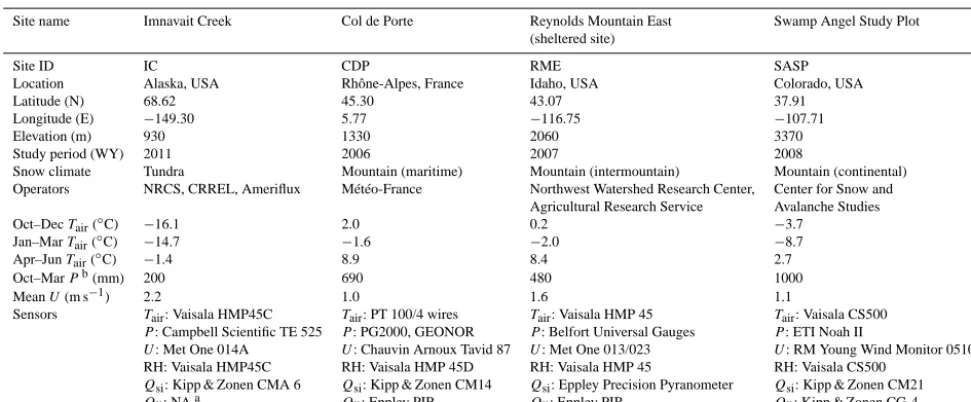
Table 1. Basic characteristics of the snow study sites, ordered from left to right by increasing elevation.

Site name Imnavait Creek Col de Porte Reynolds Mountain East Swamp Angel Study Plot (sheltered site)

Site ID IC CDP RME SASP

Location Alaska, USA Rhône-Alpes, France Idaho, USA Colorado, USA

Latitude (N) 68.62 45.30 43.07 37.91

Longitude (E) −149.30 5.77 −116.75 −107.71

Elevation (m) 930 1330 2060 3370

Study period (WY) 2011 2006 2007 2008

Snow climate Tundra Mountain (maritime) Mountain (intermountain) Mountain (continental) Operators NRCS, CRREL, Ameriflux Météo-France Northwest Watershed Research Center, Center for Snow and

Agricultural Research Service Avalanche Studies

Oct–DecTair(◦C) −16.1 2.0 0.2 −3.7

Jan–MarTair(◦C) −14.7 −1.6 −2.0 −8.7

Apr–JunT_air(◦_{C) −1.4 8.9 8.4 2.7}

Oct–MarPb(mm) 200 690 480 1000

MeanU(m s−1) 2.2 1.0 1.6 1.1

Sensors Tair: Vaisala HMP45C Tair: PT 100/4 wires Tair: Vaisala HMP 45 Tair: Vaisala CS500

P: Campbell Scientific TE 525 P: PG2000, GEONOR P: Belfort Universal Gauges P: ETI Noah II

U: Met One 014A U: Chauvin Arnoux Tavid 87 U: Met One 013/023 U: RM Young Wind Monitor 05103-5 RH: Vaisala HMP45C RH: Vaisala HMP 45D RH: Vaisala HMP 45 RH: Vaisala CS500

Qsi: Kipp & Zonen CMA 6 Qsi: Kipp & Zonen CM14 Qsi: Eppley Precision Pyranometer Qsi: Kipp & Zonen CM21

Qli: NAa Qli: Eppley PIR Qli: Eppley PIR Qli: Kipp & Zonen CG-4

a_{At IC,Q}

liwas taken asQli=Qnet−(Qsi−Qso)+(5.67×10−8_)T4

surf, whereQnetis measured net radiation (W m−2_),Q

siis measured incoming shortwave radiation (W m−2_),Q

sois measured reflected shortwave radiation (W m−2_{), andT}

surfis measured snow surface temperature (K).bNote thatPdata were adjusted with a multiplier (see Sect. 2) prior to conducting the sensitivity analysis.

2 Study sites and data

We selected four seasonally snow covered study sites (Ta-ble 1) in distinct snow climates (Sturm et al., 1995; Tru-jillo and Molotch, 2014). The sites included (1) the Im-navait Creek (IC, 930 m) site (Euskirchen et al., 2012; Kane et al., 1991; Sturm and Wagner, 2010), located in the tundra north of the Brooks Range in Alaska, USA, (2) the maritime Col de Porte (CDP, 1330 m) site (Morin et al., 2012) in the Chartreuse Range in the Rhône-Alpes of France, (3) the in-termountain Reynolds Mountain East (RME, 2060 m) shel-tered site (Reba et al., 2011) in the Owyhee Range in Idaho, USA, and (4) the continental Swamp Angel Study Plot (SASP, 3370 m) site (Landry et al., 2014) in the San Juan Mountains of Colorado, USA. We selected these sites be-cause of the quality and completeness of the forcing data and because they spanned contrasting climates (Table 1), allow-ing us to check for potential climate dependencies in sen-sitivity to forcing errors. Generalization of the results with climate was not possible due to the low sample size of sites.

The sites had high-quality observations of model forcings at hourly time steps. Serially complete published data sets are available at CDP, RME, and SASP (see citations above). At IC, data were available from multiple co-located stations (Griffin et al., 2010; Bret-Harte et al., 2010a, b, 2011b, c, a; Sturm and Wagner, 2010). These data were quality con-trolled, and gaps in the data were filled as described in Raleigh (2013).

We considered only 1 year for analysis at each site (Ta-ble 1) due to the high computational costs of the experi-ment. Measured evaluation data (e.g., snow water equivalent, SWE) at daily resolution were used only for qualitative as-sessment of model output. SWE was observed at snow

pil-lows at IC and RME. At CDP, a cosmic ray detector col-lected SWE data. At SASP, acoustic snow depth data were converted to daily SWE using density inferred from nearby Snow Telemetry (SNOTEL) (Serreze et al., 1999) sites and local snow pit measurements (Raleigh, 2013).

Before conducting the sensitivity analysis, we adjusted the available precipitation data at each site with a multiplica-tive factor to correct for potential undercatch errors (e.g., Goodison et al., 1998; Rasmussen et al., 2012; Yang et al., 2000) and to ensure the base model simulation with all ob-served forcings reasonably represented obob-served SWE. Sev-eral studies have demonstrated the necessity of precipita-tion adjustments for realistic SWE simulaprecipita-tions, even at well-instrumented sites (e.g., Hiemstra et al., 2006; Reba et al., 2011; Schmucki et al., 2014). Precipitation adjustments were most necessary at IC, where windy conditions preclude ef-fective measurements (Yang et al., 2000). In contrast, only modest adjustments were necessary at the other three sites because they were located in sheltered clearings and because some corrections were already applied to the published data. We considered adjustment multipliers ranging from 0.5 to 2.5 (increments of 0.05) and selected the multiplier that yielded the lowest root mean squared error between observed and modeled SWE. Precipitation multipliers were 1.6 at IC and 1.15 at SASP, and 0.9 at CDP and RME. The undercatch er-rors at IC were consistent with the 61–68 % of the undercatch errors found by Yang et al. (2000) for Wyoming-type gauges in wind-blown regions.

pre-cipitation multipliers was warranted. Manual observations of SWE (e.g., snow surveys, snow pits) generally supported the automatically collected SWE observations (no figures shown) and thus differences between observed and mod-eled SWE did not likely stem from issues in the verification data. Sites where we decreased the precipitation data (CDP and RME) were also the warmer sites and experienced more mixed rain–snow events in the winter. Hence, we considered multiple hypotheses to explain the SWE differences at these sites: (1) the choice of rain–snow parameterization, (2) the choice of parameters (e.g., threshold temperatures) for the rain–snow parameterization, and (3) the quality of the forc-ing data (e.g., precipitation). For these warmer sites, an ex-ploratory analysis revealed that either (1) or (3) could explain the SWE differences, but auxiliary data (e.g., precipitation phase data) were not available to discriminate these hypothe-ses. Choosing a different rain–snow parameterization might minimize the SWE differences at the warmer sites but would not rectify the SWE differences at the colder sites (IC and SASP) where most winter precipitation falls as snow. There-fore, the most straightforward and consistent approach was to adjust the precipitation data and to leave the native UEB pa-rameterizations intact. It was beyond the scope of this study to optimize model parameters and unravel the relative contri-butions of uncertainty for factors other than the meteorologi-cal forcings. Nevertheless, we suggest these precipitation ad-justments minimally affected the sensitivity analysis, as we did not quantitatively compare the model outputs to the ob-served response variables (e.g., SWE).

3 Methods

3.1 Model and output metrics

The UEB is a physically based, one-dimensional snow model (Mahat and Tarboton, 2012; Tarboton and Luce, 1996; You et al., 2014). UEB represents processes such as snow accu-mulation, snowmelt, albedo decay, surface temperature vari-ation, liquid water retention and refreezing, and sublimation. Due to the one-dimensional structure of the model, UEB does not account for lateral mass transfer of snow (e.g., wind-induced snow drifting) and therefore these processes must be represented in other model components (e.g., precipita-tion uncertainty; see Sect. 3.2.3). UEB has a single bulk snow layer and an infinitesimally thin surface layer for energy bal-ance computations at the snow–atmosphere interface. UEB tracks state variables for snowpack energy content, SWE, and a dimensionless snow surface age (for albedo computa-tions). We ran UEB at hourly time steps with six forcings: air temperature (Tair), precipitation (P), wind speed (U), relative

humidity (RH), incoming shortwave radiation (Qsi), and

in-coming longwave radiation (Qli). We used fixed parameters

across all scenarios (Table 2). We initialized UEB during the snow-free period; thus, model spin-up was unnecessary.

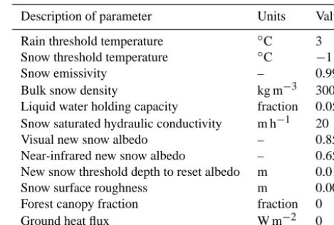
Table 2. UEB model parameters used in all simulations and sites.

Description of parameter Units Value

Rain threshold temperature ◦C 3

Snow threshold temperature ◦C −1

Snow emissivity – 0.99

Bulk snow density kg m−3 300

Liquid water holding capacity fraction 0.05 Snow saturated hydraulic conductivity m h−1 20

Visual new snow albedo – 0.85

Near-infrared new snow albedo – 0.65

New snow threshold depth to reset albedo m 0.01

Snow surface roughness m 0.005

Forest canopy fraction fraction 0

Ground heat flux W m−2 0

With each UEB simulation, we calculated four summary output metrics: (1) peak (i.e., maximum) SWE, (2) mean ab-lation rate, (3) snow disappearance date, and (4) total annual snow sublimation. The first three metrics are important for the timing and magnitude of water availability and identifi-cation of the snowpack regime (Trujillo and Molotch, 2014), while the fourth impacts the partitioning of annualP into runoff and evapotranspiration. We calculated the snow disap-pearance date as the first date when 90 % of peak SWE had ablated, similar to other studies that use a minimum SWE threshold for defining snow disappearance (e.g., Schmucki et al., 2014). The mean ablation rate was calculated in the period between peak SWE and snow disappearance and was taken as the absolute value of the mean of all SWE decreases.

3.2 Forcing error scenarios

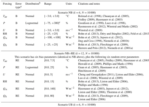
magni-Table 3. Details of error types, distributions, and uncertainty ranges for the five scenarios.

Forcing Error Distributionb Range Units Citations and notes typea

Scenario NB (k=6,N=10 000)

Tair B Normal [−3.0,+3.0] ◦C Bolstad et al. (1998), Chuanyan et al. (2005), Fridley (2009), Hasenauer et al. (2003) P B Lognormal [−75,+300]c % Goodison et al. (1998), Luce et al. (1998),

Rasmussen et al. (2012), Winstral and Marks (2002) U B Normal [−3.0,+3.0] m s−1 Winstral et al. (2009)

RH B Normal [−25,+25] % Bohn et al. (2013), Déry and Stieglitz (2002), Feld et al. (2013) Qsi B Normal [−100,+100] W m−2 Bohn et al. (2013), Jepsen et al. (2012),

Jing and Cess (1998), Niemelä et al. (2001b) Qli B Normal [−25,+25] W m−2 Bohn et al. (2013), Flerchinger et al. (2009),

Herrero and Polo (2012), Niemelä et al. (2001a)

Scenario NB+RE (k=12,N=10 000)

This scenario has six bias parameters (identical to NB above), plus the following six random error parameters

Tair RE Normal [0.0, 7.5] ◦C Chuanyan et al. (2005), Fridley (2009), Hasenauer et al. (2003), Huwald et al. (2009), Phillips and Marks (1996)

P RE Lognormal [0.0, 25] % Guan et al. (2005), Hasenauer et al. (2003), Hutchinson et al. (2009)

U RE Normal [0.0, 5] m s−1 Cheng and Georgakakos (2011), Liston and Elder (2006), Luo et al. (2008), Winstral et al. (2009)

RH RE Normal [0.0, 15] % Bohn et al. (2013), Liston and Elder (2006), Phillips and Marks (1996)

Qsi RE Normal [0.0, 160] W m−2 Hasenauer et al. (2003), Jepsen et al. (2012), Liston and Elder (2006), Thornton et al. (2000) Qli RE Normal [0.0, 80] W m−2 Bohn et al. (2013), Flerchinger et al. (2009),

Liston and Elder (2006)

Scenario UB (k=6,N=10 000)

This scenario is identical to NB, except all probability distributions are uniform

Scenario NB_gauge (k=6,N=10 000)

Identical to NB, exceptP uncertainty mimics documented differences betweenP and SWE at SNOTEL sites

P B Normal [−10,+10] ◦C Meyer et al. (2012)

Scenario NB_labd(k=6,N=10 000)

Tair B Normal [−0.30,+0.30] ◦C Vaisala HMP45 specified accuracy P B Lognormal [−3.0,+3.0]e % RM Young 52202 specified accuracy U B Normal [−0.30,+0.30] m s−1 RM Young 05103 specified accuracy RH B Normal [−3.0,+3.0] % Vaisala HMP45 specified accuracy Qsi B Normal [−25,+25] W m−2 Li-Cor 200X specified accuracy of∼5 % Qli B Normal [−15,+15] W m−2 Assumed∼5 % of mean intersite values

a_{B: bias, RE: random errors. Biases are additive (b}

i=0, Eq. 5) for all forcings exceptP, which has multiplicative bias (bi=1).bProbability distributions were truncated

in instances when introduction of errors caused non-physical forcing values (see Sect. 3.3.5).cThe high upperPbias (300 %) mimics cases where snowfall data collected in an area of drift deposition are assumed (incorrectly) to represent other basin locations.dUncertainty ranges in this scenario are based primarily on manufacturer’s specified accuracy for typical sensors deployed at SNOTEL sites (NRCS Staff, personal communication, 2013). We assume thePstorage gauge has the same accuracy as a typical tipping bucket gauge.eWe neglectPundercatch errors in the lab uncertainty scenario.

tudes by comparing NB (high forcing uncertainty) to both NB_gauge (moderate uncertainty in precipitation but high uncertainty for all other forcings) and NB_lab (low forcing uncertainty).

3.2.1 Error types

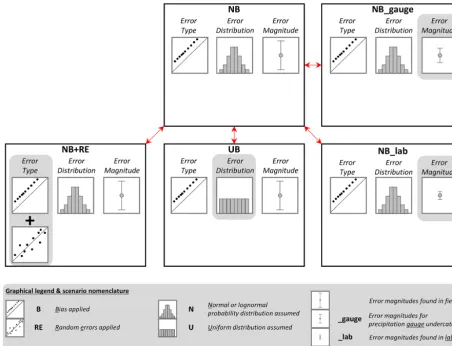
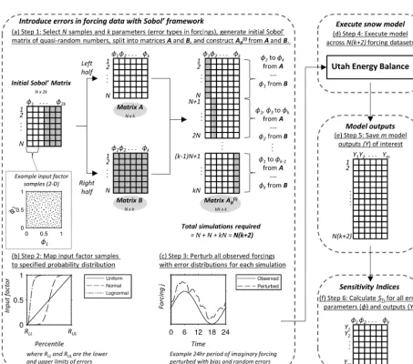
Figure 1. Scenarios of interest and the type, distribution, and magnitude of errors considered in each. NB considers normally (or lognormally)

distributed biases with error magnitudes found in the field. NB+RE is the same as NB but also considers random errors. UB is the same as NB but considers uniformly distributed errors instead. NB_gauge is the same as NB but with reduced precipitation uncertainty (typical difference between precipitation gauge and snow pillow). NB_lab is the same as NB but considers laboratory error magnitudes.

is there any consideration of interactions between these error types. As a recent example, Lapo et al. (2015) tested biases and random errors in Qsi andQli forcings, finding that

bi-ases generally introduced more variance in modeled SWE than random errors. Their experiment considered biases and random errors separately (i.e., no error interactions allowed) and examined only a subset of the required forcings (i.e., ra-diation). Here, we examined coexisting biases in all forcings in NB, UB, NB_gauge, and NB_lab, and coexisting biases and random errors in all forcings in NB+RE.

Table 3 shows the assignment of error types for the five scenarios. We relied on studies that assess errors in measure-ments or estimated forcings to identify typical characteristics of biases and random errors. Published bias values were more straightforward to interpret than random errors because com-mon metrics, such as root mean squared error (RMSE) and mean absolute error (MAE), encapsulate both systematic and random errors. Hence, when defining random errors, the pub-lished RMSE and MAE served as qualitative guidelines.

3.2.2 Error distributions

stud-ies broadly suggest that the grouping of most important fac-tors may be similar under different distribution assumptions, particularly in cases when interactions are minimal, but the relative ranking of factors within those groups may vary de-pending on the distribution. Here we test how the assumed probability distribution influences the sensitivity of a snow model to forcing errors.

We designed the UB scenario with the naive hypothesis that the probability distribution of biases was uniform for all six meteorological variables. In contrast, error distributions (Table 3) were assumed non-uniform (described below) in scenarios NB, NB+RE, NB_gauge, and NB_lab. Unfortu-nately, error distributions are reported less frequently than er-ror statistics (e.g., bias, RMSE) in the literature. We assumed thatTairand RH errors follow normal distributions (Mardikis

et al., 2005; Phillips and Marks, 1996), as doQsiandQli

er-rors. Conflicting reports over the distribution ofUindicated that errors may be approximated with a normal (Phillips and Marks, 1996), a lognormal (Mardikis et al., 2005), or a Weibull distribution (Jiménez et al., 2011). For simplicity, we assumed thatUerrors were normally distributed. Finally, we assumedP errors followed a lognormal distribution to ac-count for snow redistribution due to wind drift/scour (Liston, 2004) or to account for precipitation gauge undercatch (Du-rand and Margulis, 2007). Error distributions were truncated in cases when the introduced errors violated physical limits (e.g., negativeU; see Sect. 3.3.5).

3.2.3 Error magnitudes

We considered three magnitudes of forcing uncertainty (Ta-ble 3): levels of uncertainty found (1) in the field for all forc-ings (i.e., NB), (2) in the field for all forcforc-ings except pre-cipitation (which has uncertainty due to prepre-cipitation gauge undercatch, i.e., NB_gauge), and (3) in a controlled labora-tory setting (i.e., NB_lab). These cases were considered be-cause they sampled realistic errors (NB and NB_gauge) and minimum errors (NB_lab). We expected that the error ranges exerted a major control on model uncertainty and sensitiv-ity, as demonstrated in several prior sensitivity analyses (see review of Song et al., 2015).

Consideration of error magnitudes was achieved in each scenario by assigning a range to each error probability distri-bution (see Sect. 3.2.2 and Table 3). While non-uniform dis-tributions (e.g., normal) are typically described by measures other than the range (e.g., mean and variance), we scaled these distributions (see Sect. 3.3.5 for details) such that they were bounded within a specified range. This convention was necessary to ensure that differences between scenarios NB and UB were due solely to the shape of the error probability distributions, and not due to differences in both distribution shape and the domain. Additionally, this followed the typical practice of sensitivity analysis where the range specifies the domain of the distribution.

We considered field uncertainties in all forcings in NB, NB+RE, and UB, and in all forcings except precipitation in NB_gauge. Field uncertainties depend on the source of forcing data and on local conditions (e.g., Flerchinger et al., 2009; Lundquist et al., 2015). To generalize the analysis, we chose error ranges for the field uncertainty that enveloped the reported uncertainty of different methods for acquiring forc-ing data.Tair error ranges spanned errors in measurements

(Huwald et al., 2009) and commonly used models, such as lapse rates and statistical methods (Bolstad et al., 1998; Chuanyan et al., 2005; Fridley, 2009; Hasenauer et al., 2003; Phillips and Marks, 1996). U error ranges spanned errors in topographic drift models (Liston and Elder, 2006; Win-stral et al., 2009) and numerical weather prediction (NWP) models (Cheng and Georgakakos, 2011). RH error ranges spanned errors in observations (Déry and Stieglitz, 2002) and empirical methods (e.g., Bohn et al., 2013; Feld et al., 2013).Qsi error ranges spanned errors in empirical

meth-ods (Bohn et al., 2013), radiative transfer models (Jing and Cess, 1998), satellite-derived products (Jepsen et al., 2012), and NWP models (Niemelä et al., 2001b).Qli error ranges

spanned errors in empirical methods (Bohn et al., 2013; Flerchinger et al., 2009; Herrero and Polo, 2012) and NWP models (Niemelä et al., 2001a).

P error ranges spanned both undercatch (e.g., Rasmussen et al., 2012) and wind drift/scour errors in NB, NB+RE, and UB but only undercatch errors in NB_gauge. We assumed thatP biases due to gauge undercatch in NB_gauge ranged from−10 to+10 % because Meyer et al. (2012) found 95 % of SNOTEL sites (often in forest clearings) had observa-tions of accumulatedP within 20 % of peak SWE. Results of NB, NB+RE, and UB were thus most relevant to ar-eas with prominent snow redistribution (e.g., alpine zone), whereas NB_gauge results were more relevant to areas with minimal wind drift errors. It could be argued that uncer-tainty due to snow drift processes is a structural issue and not a source of forcing error; however, this distinction de-pends strongly on what type of model is considered. This process is clearly a structural component for snow models with explicit (e.g., three dimensional models with dynamic wind transport, Lehning et al., 2006) or implicit (e.g., one-dimensional models with probabilistic subgrid snow variabil-ity routines, Clark et al., 2011a) treatment of snow redistri-bution. However, when a one-dimensional snow model is ap-plied at length scales shorter than drift process length scales (as assumed here with UEB), it is not possible to account for snow drift in a structural sense. Therefore, we treat drifting snow as a form of precipitation error in NB, NB+RE, and UB. Because UEB lacks dynamic wind redistribution, accu-mulation uncertainty was not linked toU errors but instead toP errors (e.g., drift factor, Luce et al., 1998).

1992; Marks et al., 1992) to instrument accuracy at SASP, finding a 5-day range in uncertainty in modeled snow disap-pearance, with longwave uncertainty having the greatest im-pact. An emerging sensitivity analysis (Sauter and Obleitner, 2015) with the CROCUS model (Brun et al., 1992) applied on the Kongsvegen Glacier (Svalbard) indicates that long-wave measurement uncertainty has an approximately compa-rable effect on modeled snow depth as±25 % precipitation uncertainty and is the most dominant influence on the mod-eled energy balance and turbulent heat flux (relative to the measurement uncertainty of other forcings). Here we build on these efforts to examine how instrument accuracy impacts modeled snow variables in a variety of seasonal snow cli-mates. In reality, laboratory uncertainty levels vary with the type and quality of sensors, as well as related accessories (e.g., radiation shield for the temperature sensor), which we did not explicitly consider. Because the actual sensors avail-able varied between sites (Tavail-able 1) and we needed consistent errors across sites within scenario NB_lab, we assumed that the manufacturers’ specified accuracy of meteorological sen-sors at a typical SNOTEL site were representative of mini-mum uncertainties in forcings because of the widespread use of SNOTEL data in snow studies. While we used the spec-ified accuracy for idealizedP measurements in NB_lab, we note that the instrument uncertainty of±3 % was likely un-representative of errors likely to be encountered. For exam-ple, corrections applied to theP data (see Sect. 2) exceeded this uncertainty by factors of 3–20.

3.3 Sensitivity analysis

Numerous approaches that explore uncertainty in numeri-cal models have been developed in the literature of statistics (Christopher Frey and Patil, 2002), environmental model-ing (Matott et al., 2009), and optimization/calibration of hy-drology and earth systems models (Beven and Binley, 1992; Duan et al., 1992; Kavetski et al., 2002, 2006a, b; Kucz-era et al., 2010; Razavi and Gupta, 2015; Song et al., 2015; Vrugt et al., 2009, 2008). Among these, global sensitivity analysis is an elegant platform for testing the impact of in-put uncertainty on model outin-puts and for ranking the relative importance of inputs while considering coexisting sources of uncertainty. Global methods are ideal for non-linear models (e.g., snow models). The Sobol’ (1990) (hereafter Sobol’) method is a robust global method based on the decompo-sition of variance (see below). We investigate Sobol’, as it is often the baseline for testing sensitivity analysis methods (Herman et al., 2013; Li et al., 2013; Rakovec et al., 2014; Tang et al., 2007).

3.3.1 Overview: model conceptualization and sensitivity

One can visualize any hydrology or snow model (e.g., UEB) as

Y=M(F,θ), (1)

where Y is a matrix of model outputs (e.g., SWE),Mis the model operator, F is a matrix of forcings (e.g.,Tair,P,U),

andθ is an array of model parameters (e.g., Table 2). The goal of sensitivity analysis is to determine which input fac-tors (F and θ) are most important to specific outputs (Y) (Matott et al., 2009). Sensitivity analyses often focus more on the model parameter array (θ) than on the forcing ma-trix (Foglia et al., 2009; Herman et al., 2013; Li et al., 2013; Nossent et al., 2011; Rakovec et al., 2014; Rosero et al., 2010; Rosolem et al., 2012; Tang et al., 2007; van Werkhoven et al., 2008). However, recent analyses have considered other input factors and sources of uncertainty (e.g., Baroni and Tarantola, 2014; Schoups and Hopmans, 2006). Here, we ex-tend the sensitivity analysis framework to forcing uncertainty by creatingk new parameters (φ1,φ2, . . . ,φk) that specify

forcing uncertainty characteristics (Vrugt et al., 2008) and reformulate Eq. (1) as

Y=M(F,θ,φ). (2)

By fixing the original model parameters (Table 2), we focus solely on the influence of forcing errors on model outputs (Y). Note it is possible to consider uncertainty in both forc-ings and parameters in this framework.

3.3.2 Sobol’ sensitivity analysis

Sobol’ sensitivity analysis uses variance decomposition to at-tribute output variance to input uncertainty. First-order and higher-order sensitivities can be resolved; here, only the total-order sensitivities were examined (see below) for clar-ity and because the resulting first-order sensitivclar-ity indices were typically comparable to the total-order sensitivity in-dices (e.g., 83 % of all cases had total-order and first-order indices within 10 % of each other), suggesting minimal error interactions. The Sobol’ method is advantageous in that it is model independent, can handle non-linear systems, and is among the most robust sensitivity methods (Saltelli and An-noni, 2010; Saltelli, 1999). The primary limitation of Sobol’ is that it is computationally intensive, requiring a large num-ber of samples to account for variance across the full param-eter space. A key assumption to the Sobol’ approach used in this paper (see Sect. 3.3.3) is that the factors are independent; hence, our analysis does not consider cases of correlated er-rors (e.g., a positive measurement bias inTair that causes a

those applications for future work. Below, we provide a brief summary of the Sobol’ sensitivity analysis methodology im-plemented here but note that further details can be found in Saltelli et al. (2010).

3.3.3 Sensitivity indices and sampling

Within the Sobol’ global sensitivity analysis framework, the total-order sensitivity index (STi) describes the variance in

model outputs (Y) due to a specific forcing error (φi),

includ-ing both unique (i.e., first-order) effects and all interactions with all other parameters:

STi =

E[V (Y|φ∼i)]

V (Y) =1−

V[E (Y|φ∼i)]

V (Y) , (3)

whereEis the expectation (i.e., average) operator,V is the variance operator, andφ∼i signifies all parameters exceptφi.

The latter expression definesSTi as the variance remaining

inYafter accounting for variance due to all other parameters (φ∼i).STi values have a range of [0, 1]. Interpretation ofSTi

values was straightforward because they explicitly quantified the variance introduced to model output by each parameter (i.e., forcing errors). As an example, anSTi value of 0.7 for

bias parameterφi on outputYj indicates 70 % of the output

variance was due to bias in forcingi(including unique effects and interactions).

A number of numerical methods are available for evalu-ating sensitivity indices, and most adopt a Monte Carlo ap-proach (Saltelli et al., 2010). Evaluation of Eq. (3) requires two sampling matrices, which we refer to as matrices A and B (Fig. 2a). To construct A and B, we first specified the number of samples (N) in the parameter space and the number of parameters (k), depending on the error scenario (Table 3). Selecting input factor samples for these two ma-trices was achieved using the quasi-random Sobol’ sequence (Saltelli and Annoni, 2010). The sequence can be approx-imated as a uniform distribution in the range [0, 1]. Fig-ure 2a shows input factor samples from an example Sobol’ sequence in two dimensions. For each scenario and site, we generated a (N×2k) Sobol’ sequence matrix with quasi-random numbers in the [0, 1] range, and then divided it in two parts such that matrices A and B were each distinct (N×k) matrices. Calculation ofSTirequired perturbing

fac-tors; therefore, a third Sobol’ matrix (A(i)_B ) was constructed from A and B. In matrix A(i)_B, all columns were from A, ex-cept theith column, which was from theith column of B, re-sulting in a (kN×k) matrix (Fig. 2a). Section 3.3.5 provides specific examples of this implementation. From Eq. (3), we computeSTias (Jansen, 1999; Saltelli et al., 2010)

STi =

1 2N

N P

j=1

f (A)j−f

A(i)_B

j

2

V (Y) , (4)

where f (A) is the model output evaluated on the A ma-trix, f (A(i)_B)is the model output evaluated on the A(i)_B

ma-trix where theith column is from the B matrix, and i des-ignates the parameter of interest. Evaluation ofSTi required N (k+2) simulations at each site and scenario.

3.3.4 Bootstrapping of sensitivity indices

To test the reliability ofSTi, we used bootstrapping with

re-placement across theN (k+2) outputs, similar to Nossent et al. (2011). The mean and 95 % confidence interval were calculated using the Archer et al. (1997) percentile method and 10 000 samples. For all cases, finalSTi values (i.e.,

com-puted sensitivity indices with all samples considered) were close to the mean bootstrapped values (i.e., 99 % had a dif-ference of less than 0.001 and no difdif-ference was greater than 0.003), suggesting convergence. Thus, we report only the mean and 95 % confidence intervals of the bootstrapped

STivalues.

3.3.5 Workflow and error introduction

Figure 2 shows the workflow for creating the Sobol’ A, B, and A(i)_B matrices, mapping input factor samples to errors, ap-plying errors to the original forcing data, executing the model and saving outputs, and calculatingSTivalues. The workflow

was repeated at all sites and scenarios. Each step is described in more detail below.

– Step 1: generate an initial (N×2k) Sobol’ matrix (with

N and k values for each scenario; Table 3), separate into A and B, and construct A(i)_B (Fig. 2a). NB+RE had

k=12 (six bias and six random error parameters). All other scenarios hadk=6 (all bias parameters).

– Step 2: in each simulation, map the input factor sam-ple of each forcing error parameter (φi) to the

Figure 2. Conceptual diagram showing methodology for imposing errors on the forcings with error parameters (φi) within the Sobol’

sensitivity analysis framework, and workflow for model execution and calculation of sensitivity indices on model outputs (Y).

aQsibias parameter ofφi=0.75 (quantile value) in the

[−100 W m−2,+100 W m−2] range would map to aQsi

bias of +50 W m−2 when assuming a uniform proba-bility distribution but only+14 W m−2when assuming a normal distribution. For context, a bias parameter of +50 W m−2or higher has about a 25 % probability of occurring in the uniform distribution but only 2 % in the normal distribution.

– Step 3: in each simulation, perturb (i.e., introduce arti-ficial errors) the observed time series of theith forcing (F_i) with bias (all scenarios) or both bias and random errors (NB+RE only) (Fig. 2c):

F0_i =FiφB,ibi+ Fi+φB,i(1−bi)+φRE,iRci, (5)

whereF0_i is the perturbed forcing time series,φB,i is

the bias parameter for forcing i,bi is a binary switch

indicating multiplicative bias (bi=1) or additive bias

(bi=0),φRE,i is the random error parameter for

forc-ingi,Ris a time series of randomly distributed noise (normal distribution, mean=0) scaled in the [−1, 1] range, andci is a binary switch indicating whether

ran-dom errors are introduced (ci=1 in scenario NB+RE

andci=0 in all other scenarios). ForTair,U, RH,Qsi,

andQli,bi=0; forP,bi=1. The decision to treat

bi-ases as multiplicative forP but additive for all other forcings was made based on practical considerations (e.g., multiplicative biases inTair are difficult to

inter-pret) and on convention of past studies that report forc-ing errors. However, we note this is somewhat subjec-tive, as errors in some forcings (e.g., radiation) have been reported in both conventions. ForP,U, andQsi,

values (e.g., negativeQsi) and set these to physical

lim-its. This was most common when perturbingU, RH, and

Qsi; negative values of perturbedP only occurred when

random errors were considered (Eq. 5). Due to this re-setting of non-physical errors, the error distribution was truncated (i.e., it was not always possible to impose ex-treme errors). Additional tests (not shown) suggested that distribution truncation changed sensitivity indices minimally (i.e.,<5 %) and thus we assumed this trun-cation did not alter the relative ranking of forcing errors. – Step 4: input the N(k+2) perturbed forcing data sets into UEB (Fig. 2d). At each site, NB+RE required 140 000 simulations, whereas the other four scenar-ios each required 80 000 simulations, for a total of 1 840 000 simulations in the analysis. The doubling ofk

in NB+RE did not result in twice as many simulations because the number of simulations scaled asN (k+2). – Step 5: save the model outputs for each simulation

(Fig. 2e). The outputs included daily time series of SWE, and four summary outputs including peak SWE, mean ablation rate, snow disappearance date, and total snow sublimation.

– Step 6: calculate STi for each forcing error parameter

and model output (Fig. 2f) based on Sects. 3.3.3 and 3.3.4. Prior to calculating STi, we screened the model

outputs for cases where UEB simulated too little or too much snow (which can occur with perturbed forcings); this was an essential step to ensure meaningful results. Other studies (e.g., Pappenberger et al., 2008) have also applied screening methods to model output prior to cal-culating sensitivity indices. For a valid simulation, we required a minimum peak SWE of 50 mm, a minimum continuous snow duration of 15 days, and identifiable snow disappearance. We rejected samples that did not meet these criteria to avoid meaningless or undefined metrics (e.g., peak SWE in ephemeral snow or snow disappearance for a simulation that did not melt out). The number of rejected samples varied with site and scenario (Table 4). On average, 94 % passed the require-ments. All cases had at least 86 % satisfactory samples, except in UB at SASP, where only∼34 % met the re-quirements. In this case, the most common reason for rejecting a simulation was that too much snow was sim-ulated, such that it never disappeared by the end of the model run. The rejected runs were characterized by high (positive) precipitation biases and low (negative) biases in Tair, Qsi, andQli. Despite this attrition,STi values

still converged in all cases.

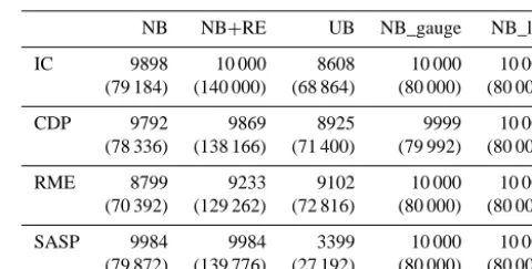
Table 4. Number of samples (N) and model simulations (in

paren-theses) meeting the requirements for minimum peak SWE and snow duration and valid snow disappearance dates at each site (rows) in each scenario (columns). The number of model simulations scaled asN(k+2), wherek=12 in scenario NB+RE andk=6 in all other scenarios. When a simulation was rejected, all related simulations (based on resampling) were also rejected.

NB NB+RE UB NB_gauge NB_lab

IC 9898 10 000 8608 10 000 10 000 (79 184) (140 000) (68 864) (80 000) (80 000)

CDP 9792 9869 8925 9999 10 000 (78 336) (138 166) (71 400) (79 992) (80 000)

RME 8799 9233 9102 10 000 10 000 (70 392) (129 262) (72 816) (80 000) (80 000)

SASP 9984 9984 3399 10 000 10 000 (79 872) (139 776) (27 192) (80 000) (80 000)

4 Results

4.1 Propagation of forcing uncertainty to model outputs

Figure 3 shows density plots of daily SWE from UEB at the four sites and five forcing error scenarios (Fig. 1, Table 3), while Fig. 4 summarizes the model outputs. As a reminder, NB assumed normal (or lognormal) biases at field level un-certainty. The other scenarios were the same as NB, except NB+RE considered both biases and random errors, UB con-sidered uniform distributions, NB_gauge concon-sidered gauge undercatch biases in precipitation, and NB_lab considered lower error magnitudes in all forcings (i.e., laboratory level uncertainty).

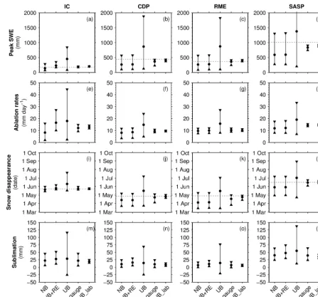
Large uncertainties in SWE were evident, particularly in NB, NB+RE, and UB (Fig. 3a–l). The large range in mod-eled SWE within these three scenarios often translated to large ranges in mean ablation rates (Fig. 4e–h), snow dis-appearance dates (Fig. 4i–l) and total sublimation (Fig. 4m– p). In contrast, SWE and output uncertainties in NB_gauge and NB_lab were comparatively small (Figs. 3m–t, 4). Model output ranges were generally larger in NB_gauge than in NB_lab. The envelope of SWE simulations in NB_lab more tightly encompassed observed SWE at all sites, except dur-ing early winter at IC (Fig. 3m), which was possibly due to initialP data quality and redistribution of snow to the snow pillow site.

Figure 3. Observed (black line) and modeled SWE (color density plot) at the four sites across the five uncertainty scenarios (see Fig. 1

and Table 3). The number of model simulations in the density plots varies with the site and scenario (see Table 4). The density plots were constructed using 100 bins in the SWE dimension with relative frequency tabulated in each bin each day. Note the frequency color bar is on a logarithmic scale. Sites are arranged from top to bottom in order of increasing elevation and decreasing latitude. Scenarios are defined as normally distributed bias (NB), normally distributed bias and random errors (NB+RE), uniformly distributed bias (UB), normally distributed bias with precipitation gauge uncertainty (NB_gauge), and normally distributed bias at laboratory error magnitudes (NB_lab).

(particularly for the ablation rates), indicating that random errors had some influence there, and this was possibly due to the low snow accumulation (∼200 mm peak SWE observed) at that site and brief snowmelt season (less than 10 days in the observations).

NB and UB yielded generally very different model out-puts (Figs. 3, 4). The only difference in these two scenar-ios was the assumption regarding error distribution (Table 3). Uniformly distributed forcing biases (scenario UB) yielded a relatively uniform ensemble of SWE simulations (Fig. 3i–l), larger mean values of peak SWE and ablation rates, and later snow disappearance, as well as larger uncertainty ranges in

all outputs (Fig. 4). At some sites, UB also had a higher fre-quency of simulations where seasonal sublimation was neg-ative (i.e., condensation).

Figure 4. Distributions of model outputs (rows) at the four study sites (columns) arranged by scenario. For each scenario, the circle is the

mean and the whiskers show the range encompassing 95 % of the simulations (see Table 4 for number of simulations for each site and scenario). The dashed lines in (a)–(d) and (i)–(l) are the observed values. Axes are matched between sites for a given model output; note that the range in scenario UB in (d) is truncated by the axes’ limits (upper value=3030 mm).

Relative to NB, NB_lab had smaller uncertainty ranges in all model outputs (Figs. 3, 4), an expected result given the lower magnitudes in forcing errors in NB_lab (Table 3). Likewise, NB_lab SWE simulations were generally less bi-ased than NB, relative to observations (Fig. 3). NB_lab gen-erally had higher mean peak SWE and ablation rates and later mean snow disappearance timing than NB (Fig. 4).

4.2 Model sensitivity to forcing error characteristics Total-order sensitivity indices (STi) were calculated for four

summary variables of model output (peak SWE, mean abla-tion rates, snow disappearance dates, and total sublimaabla-tion) and for daily SWE output at all sites and error scenarios.

Ex-amination of the total-order indices with sample size indi-cated that most indices stabilized after evaluating the model at 3000–5000 samples (no figures shown). Below we sequen-tially compare sensitivity indices from different scenarios to scenario NB to test the impact of differences in error charac-teristics (type, probability distribution, and magnitudes).

4.2.1 Impact of error types

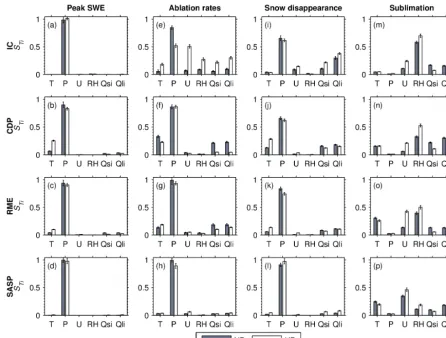
Figure 5. Model sensitivity as a function of forcing error type. Shown are the total-order sensitivity indices (STi) of four model response

variables (columns) at the four sites (rows) from scenarios NB and NB+RE. In NB+RE, bias and random error parameters are shown separately. NB+RE considers normally distributed bias and random errors, while NB considers normally distributed bias only. The bar indicates the mean (bootstrapped) sensitivity indices and associated 95 % confidence intervals.

UEB peak SWE was most sensitive to P bias at all sites (Fig. 5a–d). In both scenarios,P bias was also the most im-portant factor for ablation rates and snow disappearance at all sites (Fig. 5e–l). For ablation rates in NB, Tair bias was

the next most important factor (afterP bias) at CDP, while biases in Qsi andQli were secondarily important at RME

(Fig. 5f, g). For ablation rates at IC in NB+RE, most types of errors had some baseline influence (i.e.,STi=0.5) on model

sensitivity (Fig. 5e). In both NB and NB+RE, biases in the radiation terms were of secondary importance to snow dis-appearance timing (Fig. 5i–k). In contrast to the other three model outputs, sublimation in NB and NB+RE was insen-sitive toP bias and the most important factors varied some-what between sites and scenarios (Fig. 5m–p). In both sce-narios, sublimation was most sensitive to RH bias at IC and

U bias at SASP. At CDP and RME, sublimation was most sensitive to RH bias in NB; however, in NB+RE, sublima-tion was most sensitive to Qli bias at CDP and to Tair bias

at RME (Fig. 5n, o). In both scenarios, biases inTair,Qsi, or

Qliwere generally of secondary importance for sublimation.

We hypothesized that the snow model outputs would have higher sensitivity to biases than to random errors in the forc-ings. The results of our analysis generally supported this hy-pothesis. Across all outputs and sites,STi values for random

errors were always less than or comparable to the small-estSTi bias values, and the most important factor was

al-ways a bias term (Fig. 5). Furthermore, there was typically high correspondence between NB and NB+RE (bias terms only) in terms of identifying the most important forcing er-ror (e.g.,P bias in peak SWE and ablation rates at all sites, Fig. 5a–h). The main exceptions were snow disappearance at IC (Fig. 5i), and sublimation at CDP and RME (Fig. 5n, o), where the two scenarios identified different errors as the most important factor. However, even in these exceptional cases, the two scenarios yielded similar groupings of more important vs. least important errors. For example, biases in

scenarios (Fig. 5o), though they distinguished these sensitiv-ities differently (i.e., NB found the RH bias was more impor-tant whereas NB+RE found theTair bias was more

impor-tant).

While there was general correspondence between NB and NB+RE (bias terms), sensitivity indices were not identical across cases, due to interactions between biases and random errors in NB+RE. Random errors changed model sensitiv-ity to biases, and the change in sensitivsensitiv-ity was more notable (i.e., absolute change exceeding 0.10) for ablation rates and snow disappearance at IC (Fig. 5e, i) and sublimation at all sites (Fig. 5m–p). Random errors amplified model sensitiv-ity to biases in some cases (e.g., U bias in all sublimation scenarios) but diminished model sensitivity to biases in other cases (e.g., RH bias in all sublimation scenarios). Because consideration of second-order sensitivity indices was beyond the scope of the study, we were unable to determine which specific interactions were important in terms of error types, and leave this topic for future work.

4.2.2 Impact of probability distribution of errors

We hypothesized that the assumed probability distribution of errors would alter the relative hierarchy of forcing biases. However, the results did not consistently support this hypoth-esis (Fig. 6). In all cases, scenarios NB and UB identified the same factor as the most important and similar factors as the least important at all sites. Specifically,P bias was most important for peak SWE, ablation rates, and snow disappear-ance at all sites in both scenarios (Fig. 6a–l). The only ex-ception was in scenario UB at IC, where ablation rates had similar sensitivity toP bias andU bias. In both scenarios,

Tairbias was the second most important factor for peak SWE

and ablation rates at the warmest site, CDP. Both scenarios showed that RH bias was the least important factor to snow disappearance at all four sites (Fig. 6i–l). Finally, both NB and UB showed that P bias was least important for subli-mation (in contrast to the other model outputs) and that RH andUbiases were among the most sensitive factors for subli-mation (Fig. 6m–p). More specifically, sublisubli-mation was most sensitive to RH bias at IC, CDP and RME, and toU bias at SASP (Fig. 6m–p).

For a few specific forcings and outputs, the selected prob-ability distribution played a role in model sensitivity to that type of forcing bias. For example, assumption of a uniform probability distribution (UB) for forcing errors enhanced the sensitivity of sublimation to U and RH biases but re-duced sublimation sensitivity to Qsi and Qli biases at all

sites (Fig. 6m–p). In contrast, assuming a normal distribu-tion (NB) of biases yielded the opposite results. Addidistribu-tionally, modeled ablation rates at IC were notably more sensitive to forcing biases (precipitation excluded) in scenario UB than in NB.

4.2.3 Impact of error magnitude

We hypothesized that the relative magnitude of forcing errors would exert a strong control on model sensitivity. Compar-ing NB to NB_gauge and to NB_lab generally supported this hypothesis (Fig. 7). The contrast inSTi values between

sce-narios NB, NB_gauge, and NB_lab implied that the specified ranges of forcing errors was a critical determinant of model sensitivity.

WhileP bias was the most important factor at all sites in NB for peak SWE, ablation rates, and snow disappearance,P

bias was never the most important factor for these model out-puts in NB_gauge and in many cases was among the least im-portant errors (Fig. 7a–l). In NB_gauge, peak SWE was most sensitive to RH bias at IC, toTairbias at CDP and RME, and

toQlibias at SASP (Fig. 7a–d). Ablation rates in NB_gauge

were most sensitive to Tair bias at CDP and toQli bias at

IC, RME, and SASP (Fig. 7e–h). Snow disappearance was also most sensitive toQli bias at all four sites in NB_gauge

(Fig. 7i–l). However, for sublimation at all sites, NB and NB_gauge yielded very similar sensitivities to forcing bi-ases (Fig. 7m–p). Specifically, in both NB and NB_gauge, modeled sublimation was most sensitive to RH bias at IC, CDP, and RME and to U bias at SASP (Fig. 7m–p). The similarity in sublimation sensitivity indices between NB and NB_gauge emerged because these scenarios only differed in terms ofP uncertainty (Table 3) and becauseP bias was not important to modeled sublimation. The contrast between sensitivity indices in these two scenarios and for these four outputs illustrated that model sensitivity may depend on both the magnitudes of uncertainty for specific forcings and on the output of interest.

Whereas NB_gauge demonstrated that reducing the mag-nitude of forcing uncertainty in one factor (i.e., precipita-tion) was sufficient to change which factors were most and least important, NB_lab showed that changing the magni-tude of forcing uncertainty in all terms could yield a sub-stantially different pattern of model sensitivity (Fig. 7). As a primary example, scenarios NB and NB_lab did not agree on whetherP bias orQlibias was the most important factor for

peak SWE, ablation rates, and snow disappearance dates at all four sites (Fig. 7a–l). For sublimation, NB_lab sensitivity indices indicated thatQlibias was most important, whereas

RH bias (IC, CDP, and RME) andUbias (SASP) were most important in NB (Fig. 7m–p). Across all sites and outputs in NB_lab,Qli bias was consistently the most important

fac-tor (Fig. 7). In one sense, this was surprising, given that the bias magnitudes were lower forQli than forQsi(Table 3).

However, the albedo of snow minimizes the amount of en-ergy transmitted to the snowpack fromQsi, thereby

render-ingQsi errors less important than Qli errors. Additionally,

the non-linear nature of the model may enhance the role of

Qlithrough interactions with other factors. The general lack

Figure 6. Same as Fig. 5, but comparingSTi values from scenarios NB and UB to test model sensitivity as a function of error probability

distribution. UB considers uniformly distributed bias, while NB considers normally distributed bias.

laboratory-specified accuracy forP gauges and typical errors encountered in the field.

4.2.4 Relative controls of forcing error characteristics on SWE sensitivity

The above results sequentially compared sensitivity indices from different error scenarios to NB in order to ascertain how different assumptions regarding error types, probability distributions, and magnitudes translated to changes in model sensitivity. To summarize the relative controls of these three forcing error characteristics on model sensitivity, we calcu-lated daily sensitivity indices of modeled SWE to forcing bi-ases at each site and scenario (Fig. 8). This final analysis was conceptually different than the previous analyses (Figs. 5–7) in terms of the model output considered. Whereas the pre-vious analyses computed sensitivity indices for summative model outputs (e.g., peak SWE, total sublimation), the final analysis recalculated sensitivity indices for SWE each day. This approach allowed us to examine how SWE model sen-sitivity changed as a function of time within the snow season.

Comparing the broad patterns in the time varyingSTi

val-ues across the five scenarios, it was evident that error mag-nitudes were the greatest determinant in model sensitivity to forcing errors through the snow season (compare Fig. 8a–l with m–t). NB, NB+RE, and UB exhibited similar patterns, with high STi in P bias throughout the year and with the

other forcing biases yielding lowSTi values in the winter

and increasing STi values in the spring and early summer

for some forcings (Fig. 8a–l). In contrast, NB_gauge and NB_lab (Fig. 8m–t) had lowerSTivalues forP bias and more

coherent changes inSTi values that were more synchronized

with the specific part of the snow season.

After error magnitudes, the next most important determi-nant to model sensitivity was the probabilistic distribution of forcing errors (compare Fig. 8a–d and i–l). Relative to NB, UB tended to yield lowerSTi values forP bias. UB also had

higherSTivalues for biases inTair,Qli, andQsias time

pro-gressed at IC, CDP, and RME (Fig. 8i–k). Finally, the ad-dition of random errors was least important to model sensi-tivity, as the evolution ofSTi bias values was very similar

Figure 7. Same as Fig. 5, but comparingSTi values from scenarios NB, NB_gauge, and NB_lab to test model sensitivity as a function

of error magnitudes. NB considers normally distributed bias at error magnitudes found in the field. NB_gauge has lower precipitation uncertainty (gauge undercatch) than NB but is otherwise identical. NB_lab considers normally distributed bias at error magnitudes found in the laboratory.

and e–h). Random errors mattered the most to modeled SWE at IC, but random errors only changed STi values (on

aver-age) by less than 10 %.

5 Discussion

Here we examined the sensitivity of physically based snow simulations to forcing error characteristics (i.e., types, proba-bility distributions, and magnitudes) using the Sobol’ global sensitivity analysis. A key result is that among these three characteristics, the magnitude of biases had the most signifi-cant impact on UEB simulations (Figs. 3, 4) and on model sensitivity (Figs. 7, 8). The assumed probability distribu-tion of biases was important in that it increased the range of model outputs (compare NB and UB in Fig. 4) but, sur-prisingly, this usually translated to only modest changes in model sensitivity to forcing errors (Figs. 6, 8). Random er-rors were usually less important than biases. Although ran-dom errors changed model sensitivity to biases through error

interactions, this effect was only large in specific conditions (e.g., ablation rates at IC; Fig. 5e), and the snow model was never more sensitive to random errors than to biases (Fig. 5). Below we discuss these three error characteristics (in order of importance, as suggested by the results), place forcing un-certainty in the context of structural unun-certainty, and identify limitations of the analysis and future research directions.

5.1 Ranges of error magnitudes

The results supported our hypothesis that the magnitude of biases strongly influences the relative importance of forc-ing errors. The three magnitudes of uncertainty considered (NB, NB_gauge, and NB_lab) all resulted in different terns in model sensitivity to forcing biases, and these pat-terns also varied with the output of interest (Fig. 7). Mod-eled peak SWE, ablation rates, and snow disappearance were consistently sensitive toP bias in scenario NB and to Qli

sce-Figure 8. Variation of daily SWE sensitivity to forcing bias based on site (columns) and error scenario (rows). The normalized range (where

1=maximum SWE) in modeled SWE is shown (gray area) for context. Sensitivity indices in the early and late part of the snow season were screened out, as a high number of simulations with SWE=0 yielded invalid sensitivity indices.

nario NB_gauge. While peak SWE, ablation rates, and snow disappearance dates had similar sensitivities to forcing er-rors (particularly toP biases), sublimation exhibited notably different sensitivity to forcing errors.P bias was frequently

the least important factor for sublimation, in contrast to the other model outputs. Biases in RH,U, andTair were often

sub-limation in NB_lab. These field results partially agree with the sensitivity analysis of Lapp et al. (2005), who showed the most important forcings for sublimation in the Canadian Rockies wereUandQsi. However, they did not considerQli

in their sensitivity analysis, so the experiments are not ex-actly comparable. These results suggest that no single forc-ing is important across all modeled variables and that model sensitivity strongly depends on the output of interest.

The dominant effect ofP bias on modeled peak SWE, ab-lation rates, and snow disappearance in the field scenarios (e.g., NB) confirmed previous reports thatP uncertainty is a major control on snowpack dynamics (Durand and Margulis, 2008; He et al., 2011a; Schmucki et al., 2014). It was sur-prising thatP bias was often the most critical forcing error for ablation rates in these scenarios (Figs. 5, 6). Prior inves-tigations into the relative importance of forcings to ablation were typically framed for a snowpack at the end of winter, such thatP uncertainty was not considered (e.g., Zuzel and Cox, 1975). The results here showed that ablation rates were highly sensitive toP bias and this is likely because it con-trolled the timing and length of the ablation season. Posi-tiveP bias extends the fraction of the ablation season in the warmest summer months when ablation rates and radiative energy approach maximum values, whereas negativeP bias truncates the fraction of ablation in the warm season. Tru-jillo and Molotch (2014) reported a similar result based on SNOTEL observations.

The contrast between scenarios NB, NB_gauge, and NB_lab highlights that selection of the error ranges is a critical step in sensitivity analysis. However, we recognize that there is some subjectivity in the specification of these ranges. Quantification of errors in forcing estimation meth-ods is best achieved through comparisons with surface ob-servations (e.g., Bohn et al., 2013; Flerchinger et al., 2009), but it remains challenging to specify error ranges with con-fidence (Song et al., 2015). Key considerations controlling the ranges and impacts of forcing errors include the repre-sentativeness of the forcing data (e.g., reanalysis, numerical weather model output, extrapolated surface measurements) in the study area, the length scale of dominant processes (e.g., snow drifting), and the configuration of the snow model (e.g., spatial scale, complexity). Here we selected ranges in the field scenarios to encompass errors encountered across a variety of possible forcing data sources (Table 3), but ulti-mately the appropriate ranges must be tailored to the specific application. This supports the need for continual evaluation of forcing data sets across a variety of climates and environ-mental conditions.

5.2 Probability distribution of errors

The results did not universally support our hypothesis that the assumed probability distribution of biases was important to the relative ranking of forcing errors. The relative consis-tency in the dominant forcing errors between NB and UB

may have emerged because the probability distributions of all six forcing biases varied together between these two sce-narios (i.e., all forcing biases were uniform in UB and either normal or lognormal in NB). While we did not conduct addi-tional tests, we suspect that changing the probability distribu-tion of just a single forcing error (e.g.,Tairbias) from normal

to uniform would have uniquely enhanced model sensitivity to that particular forcing error (Touhami et al., 2013).

The similarity of results between scenarios NB and UB conform to findings in previous studies (e.g., Foscarini et al., 2010; Touhami et al., 2013) where uniform and normal dis-tributions identified similar factors as the most important. These previous studies imply that greater differences in sen-sitivity indices (as a function of distribution) will emerge when factor interactions are more prominent. The case with the strongest error interactions here (i.e., ablation rates at IC) also yielded the largest differences in sensitivity indices be-tween scenarios NB and UB, which is consistent with the prevailing logic.

5.3 Error types

The results were consistent with our hypothesis that the snow model is more sensitive to biases than to random er-rors in the forcings. While previous investigations supported this idea for shortwave and longwave forcings in physically based snow models (i.e., Lapo et al., 2015), the current study showed that biases are more important than random errors for all commonly required meteorological forcings (and not just irradiances). The model was more sensitive to biases and less sensitive to random errors due to the systematic nature of biases. In contrast, the effect of random errors tended to cancel out when integrating model outputs over long peri-ods. Our selected model outputs were generally a function of several months of mass and energy exchange in the snow-pack, thereby ensuring minimization of effects from random errors. Random errors only had a greater impact on ablation rates at IC (Fig. 5e) and this was because the relatively brief snowmelt period presented an opportunity for the random er-rors to not cancel out. Hence, the model may have greater sensitivity to random errors for other model outputs not con-sidered here that integrate over relatively short timescales (e.g., snowmelt over a single day).

5.4 Contextualizing forcing and structural uncertainties

Figure 9. Uncertainty ranges (95 % intervals) in (a) peak SWE, (b) ablation rates, and (c) snow disappearance date at CDP in

WY2006 for three forcing uncertainty scenarios and the Essery et al. (2013) structural uncertainty.

snow cover fraction, snow hydrology, and thermal conductiv-ity) on SWE simulations from 1701 physically based snow models at the same site/year. Figure 9 compares the 95 % uncertainty ranges in peak SWE, ablation rates, and snow disappearance in NB, NB_gauge, and NB_lab to the ranges found across the 1701 snow models of Essery et al. (2013). From the comparisons at this site, it is clear that the un-certainty associated with drifting snow (i.e., scenario NB) overwhelms the structural uncertainty in local snowpack pro-cesses for all three model outputs. As discussed previously, it could be argued that the uncertainty due to drifting snow is a structural issue (not a forcing issue) and that this does not represent the uncertainty of sheltered areas where drift-ing snow is less important. Hence, NB_gauge may be a better determinant of the level of uncertainty that can be attributed unambiguously to errors in forcing data. In that case, the out-put uncertainty range due to model forcing is still larger than that due to the structural uncertainty (as considered by Essery et al., 2013) in the cases of peak SWE and snow disappear-ance but is smaller for ablation rates (Fig. 9). As expected, the case of forcing uncertainty in NB_lab yields the lowest range in model outputs at CDP (Fig. 9), though it is interest-ing to note that the uncertainty in peak SWE due to structural uncertainty (90 mm) is only marginally larger than that due to the specified instrument accuracy (60 mm). These

compar-isons illustrate that forcing uncertainty cannot be discounted and that the magnitude of forcing uncertainty is a critical fac-tor in how forcing uncertainty compares to other sources of uncertainty (e.g., structural). This resonates with the recent work of Magnusson et al. (2015), who found that uncertainty in theP forcing was a greater determinant of model perfor-mance than structural considerations.

5.5 Caveats and future research

Limitations of the analysis are that the impact of forcing er-ror characteristics on model behavior is evaluated through the lens of a single sensitivity analysis method and a single snow model. It is possible that alternative sensitivity anal-ysis methods might yield different results than the Sobol’ method, as suggested in previous studies (e.g., Pappenberger et al., 2008). Likewise, we recognize it is possible that dif-ferent snow models may yield difdif-ferent sensitivities to forc-ing uncertainty. As one example, both Koivusalo and Heik-inheimo (1999) and Lapo et al. (2015) found UEB (Tarboton and Luce, 1996) and SNTHERM (SNow THERmal Model) (Jordan, 1991) exhibited significant differences in radiative and turbulent heat exchange. As another example, the role of U bias on snowpack formation may vary strongly de-pending on the snow model configuration. Because of the lack of wind transport in UEB, we lumped snow drift un-certainty intoP uncertainty via a “drift factor” formulation (Luce et al., 1998) and this could not account for the role of wind in snow drift/scour processes (Mott and Lehning, 2010; Winstral et al., 2013). This convention would be unneces-sary for a model that explicitly models this process (e.g., the SNOWPACK model, Lehning et al., 2006), and for this type of model we would expect the role ofU bias to be en-hanced (relative to UEB) for outputs such as peak SWE and snow disappearance timing. While sensitivity may vary with model selection in these examples, there is also evidence sug-gesting that similar results may emerge when using differ-ent snow models for a similar type of error scenario. Despite using different models, a somewhat different suite of forc-ing variables, and slightly different error ranges, our NB_lab experiment corroborated independent reports thatQli

mea-surement uncertainty was the most important to both mod-eled snow disappearance (Skiles et al., 2012) and sublima-tion/latent heat exchange (Sauter and Obleitner, 2015). Our analysis demonstrated this result was consistent across four snow climates and this result was apparent in four different model outputs (Fig. 7). The implication here is that more work is needed to better understand how different snow mod-els respond to forcing uncertainty.