Hydrol. Earth Syst. Sci., 17, 1133–1148, 2013 www.hydrol-earth-syst-sci.net/17/1133/2013/ doi:10.5194/hess-17-1133-2013
© Author(s) 2013. CC Attribution 3.0 License.
EGU Journal Logos (RGB)
Advances in
Geosciences
Open Access
Natural Hazards
and Earth System
Sciences
Open AccessAnnales
Geophysicae
Open AccessNonlinear Processes
in Geophysics
Open AccessAtmospheric
Chemistry
and Physics
Open AccessAtmospheric
Chemistry
and Physics
Open Access DiscussionsAtmospheric
Measurement
Techniques
Open AccessAtmospheric
Measurement
Techniques
Open Access DiscussionsBiogeosciences
Open Access Open Access
Biogeosciences
Discussions
Climate
of the Past
Open Access Open Access
Climate
of the Past
Discussions
Earth System
Dynamics
Open Access Open Access
Earth System
Dynamics
DiscussionsGeoscientific
Instrumentation
Methods and
Data Systems
Open Access
Geoscientific
Instrumentation
Methods and
Data Systems
Open Access DiscussionsGeoscientific
Model Development
Open Access Open Access
Geoscientific
Model Development
DiscussionsHydrology and
Earth System
Sciences
Open AccessHydrology and
Earth System
Sciences
Open Access DiscussionsOcean Science
Open Access Open Access
Ocean Science
Discussions
Solid Earth
Open Access Open Access
Solid Earth
Discussions
The Cryosphere
Open Access Open Access
The Cryosphere
Discussions
Natural Hazards
and Earth System
Sciences
Open Access
Discussions
A generalized Damk¨ohler number for classifying material
processing in hydrological systems
C. E. Oldham1, D. E. Farrow2, and S. Peiffer3
1School of Environmental Systems Engineering, The University of Western Australia, 35 Stirling Hwy,
6009 Crawley, Western Australia
2Mathematics and Statistics, Murdoch University, 6150 Murdoch, Western Australia 3Department of Hydrology, University of Bayreuth, Bayreuth, Germany
Correspondence to: C. E. Oldham ([email protected]), D. E. Farrow ([email protected]),
and S. Peiffer ([email protected])
Received: 15 August 2012 – Published in Hydrol. Earth Syst. Sci. Discuss.: 18 September 2012 Revised: 1 February 2013 – Accepted: 17 February 2013 – Published: 15 March 2013
Abstract. Assessing the potential for transfer of pollutants
and nutrients across catchments is of primary importance under changing land use and climate. Over the past decade the connectivity/disconnectivity dynamic of a catchment has been related to its potential to export material; however, we continue to use multiple definitions of connectivity, and most have focused strongly on physical (hydrological or hy-draulic) connectivity. In contrast, this paper constantly fo-cuses on the dynamic balance between transport and mate-rial transformation, and defines matemate-rial connectivity as the effective transfer of material between elements of the hydro-logical cycle. The concept of exposure timescales is devel-oped and used to define three distinct regimes: (i) which is hydrologically connected and transport is dominated by ad-vection; (ii) which is hydrologically connected and transport is dominated by diffusion; and (iii) which is materially iso-lated. The ratio of exposure timescales to material process-ing timescales is presented as the non-dimensional number,
NE, whereNE is reaction-specific and allows estimation of
relevant spatial scales over which the reactions of interest take place. Case studies within each regime provide exam-ples of howNE can be used to characterise systems
accord-ing to their sensitivity to shifts in hydrology and gain insight into the biogeochemical processes that are signficant under the specified conditions. Finally, we explore the implications of theNE framework for improved water management, and for our understanding of biodiversity, resilience and chemical competitiveness under specified conditions.
1 Introduction
Assessing the potential for export of nutrients and pollutants from catchments is of primary importance under changing land use and climatic conditions (Pringle, 2003a), yet our ability to predict export relies on a detailed understanding of both the transport and biogeochemical processing taking place (Hornberger et al., 2001). One of the challenges for the prediction of material transfer through catchments is the high degree of heterogeneity (of source distributions, trans-port media and biogeochemical processes), and its depen-dence on scale. Dooge (1986) suggested that scaling issues were fundamental to the development of hydrological the-ory, specifically the development of scaling relations across catchment scales and up-scaling from small-scale processes (Battiato and Tartakovsky, 2011). Since that time there has been substantial research on small-scale process-based dis-tributed model descriptions, however the application of these models to large catchments has at times been problematic and the preferred modes of investigation continue to vary across scales (Table 1).
Table 1. Different preferred modes of investigation used for different scales of elements in hydrological systems.
Soil pore scale Superficial Vegetation scale Riparian scale Catchment scale aquifer scale
Vertical length scale O(mm–cm) O(m–10 m) O(10 cm–1 m) O(10 cm–1 m) O(1–10 m) Horizontal length scale O(mm–cm) O(10 m–100 km) O(10 cm–1 m) O(10–100 m) O(10–1000 km) Timescale O(min) O(days–decades) O(min–seasons) O(h–yr) O(days–decades) Typical modes of investigation Laboratory/numerical Numerical/field Laboratory/field Field/numerical Numerical/field
hydrological spatial organization, yet continued to use a hy-drological lens, via a water balance approach, to characterise systems across scales. An alternative approach is to adopt a dual lens, in which the focus remains on the dynamic bal-ance between hydrological and ecological processes. A sin-gle lens approach assumes the ecosystem responds to hydro-logical forcing; a dual lens approach assumes the ecosystem responds to shifts in the balance between hydrological and ecological processes. The range of ecological processes of relevance to catchment studies is vast; hereon we focus on material fate as expressed by biogeochemical reactions.
In an attempt to identify parameters that resolved the “scale” issue, Vach´e and McDonnell (2006) flagged that wa-ter residence times were integrative and meaningful across all scales, and went on to highlight the challenges in character-ising flow paths, and therefore residence times, that were of relevance to material transport; the residence time is a critical parameter within the dual lens approach. The residence time distribution (RTD) has been used as fundamental character-istic of aquatic systems with free surfaces (Carleton, 2002; Werner and Kadlec, 2000) and more recently of catchments (Beven, 2001; McDonnell et al., 2010; McGuire and Mc-Donnell, 2006). Botter et al. (2011) highlighted the differ-ence between the probability density function (pdf) of wa-ter parcel travel/transit time within a catchment, and the pdf of catchment residence times. They also noted the temporal variability of these pdfs as a function of meteorological and hydrological forcing (Botter et al., 2010; Hrachowitz et al., 2010). All of these authors noted the importance of the resi-dence and transit times, or their distributions, for the export of pollutants and nutrients from catchments, and recently, Basu et al. (2011a,b) explored the relationships between pdfs and pollutant and nutrient export from catchments, whereas Thompson et al. (2011a) used ratios of the coefficients of variation of chemical concentration and discharge to classify chemical export from catchments.
Estimates of characteristic residence times have been used in dimensionless ratios (Carleton, 2002; Hornberger et al., 2001; Ocampo et al., 2006) to improve our understanding of catchment hydro-chemical responses and chemical cycling. The dimensionless Damk¨ohler number, Da, has been used extensively in the discipline of chemical engineering to clas-sify a system according to the balance between transport and reaction, and is given as
Da= τT
τR (1)
whereτTis the transport (or residence) timescale andτRis the reaction timescale. Thus, Da can be considered an impor-tant non-dimensional number within the dual lens approach. Michalak and Kitanidis (2000) used Da to characterise the appearance of chemical sorption peaks in simulation exper-iments. Wehrer and Totsche (2003) used Da to characterise when breakthrough of contaminants took place under non-equilibrium conditions, Ocampo et al. (2006) explored the removal of nitrate by riparian zones and demonstrated that 50 % nitrate removal occurred when Da<1 and increased to nearly 100 % at Da = 2–20. Kurtz and Peiffer (2011) demon-strated that surface complexation needs to be considered to explain the increase of FeOOH turnover rates, by dis-solved S (II), with increasing Da numbers. Battiatoc and Tartakovsky (2011) used Da in combination with multiple scale expansions to upscale from micro (pore) scale reaction-diffusion-advection processes to derive macro (averaged) governing equations.
The residence time distributions, as explored by Botter et al. (2011), create a Damk¨ohler number distribution (DND) for a given aquatic system and Carleton (2002) explored the relationship between RTD and the DND in a wetland treatment system. In an exploration of hydrological versus biogeochemical controls, Basu et al. (2011b) used ratios of transport to reaction timescales to characterise nutrient and pollutant export from agricultural catchments. While Basu et al. (2011b) did not specifically define their regimes in terms of Da, their approach is similar. Given that the Da and the DND have been successfully used to characterise the transfer of material under a range of transport conditions and across a range of spatial scales from pores to wetlands and riparian zones, we suggest that Da could be used to characterise hy-drological elements in a catchment. We note, however, that by definition the use of Da assumes hydrological (or hy-draulic) connectivity.
the connectivity/disonnectivity dynamic (Ali and Roy, 2010; Meerkerk et al., 2009; Michaelides and Chappell, 2009; Tetzlaff et al., 2007). Pringle (2003b) noted the variety of definitions of connectivity, used across and within disci-plines. In recent years, a commonly used definition is the ability of energy, matter and organisms to transfer within and between elements (for example sub-catchments, ripar-ian zones, wetlands, streams) of the hydrologic cycle (Detty and McGuire, 2010; Pringle, 2003b). We note the historical tendency to define connectivity in terms of water movement, i.e. hydrological or hydraulic connectivity, however under this definition quantifying the threshold of hydrological dis-connectivity remains problematic. Are hydrological elements that are partially or fully saturated (with water) considered connected? Does hydrological connectivity imply transport between hydrological elements? If so, is there a minimum transit time between hydrological elements, below which the elements are considered disconnected? Hydrological connec-tivity, within these contexts and across different scales, is thus operationally defined.
Additional complexity arises when we are interested in the fate of reactive material being transferred across hydrolog-ically connected landscapes. To our knowledge there have been no attempts in the hydrological literature to charac-terise connectivity in terms of the effectiveness of transfer-ring material. Such a characteristic might be termed “mate-rial connectivity” and must take into account both the hydro-logical/hydraulic transport and the biological and/or chem-ical fate or processing; such a definition is needed under a dual lens approach. Multiple elements of the hydrological cy-cle may be fully connected hydrologically, yet if material is being removed, or settles under gravity, the material trans-fer between elements is not effective, so by our definition above, the material connectivity between those elements is poor. The effectiveness of material connectivity is a critical parameter for ecological processes and outcomes.
To illustrate our point we present two examples. Firstly, we take the example of Fe(II)-rich anoxic groundwaters being discharged into a well-oxygenated stream which then flows into a lake. The groundwater, stream and lake are hydro-logically and hydraulically fully connected; however, Fe(II) undergoes oxidation on exposure to oxygenated waters, and likely precipitates as Fe(III)-oxide, which may affect the ben-thic ecology. The balance between the rate of transport, the rate of Fe(II) oxidation, the rate of precipitation and set-tling, and the rate of Fe(II) production from reductive disso-lution will determine the effectiveness of material connectiv-ity, with respect to Fe(II), between the groundwater and lake. If all Fe(II) is oxidized before reaching the lake, the systems are materially disconnected with respect to Fe(II). Under this scenario, the reaction timescale (oxidation, precipitation and settling) is much shorter that the transport timescale, Da1, ensuring material disconnectivity even under hydrologically connected conditions. Secondly, we take the example of a phytoplankton-rich wetland under flooding conditions, being
flushed out across a floodplain and into a lake. The wetland, the floodplain and the lake are hydraulically connected, how-ever in transit the phytoplankton may grow, aggregate, settle and decompose. The balance between the rate of transport, the rate of particle settling under gravity and the phytoplank-ton net productivity will determine the extent of material con-nectivity, with respect to the phytoplankton, between the wet-land and the lake. If all phytoplankton settle out (or decom-pose) before reaching the lake, the lake and wetland are ma-terially disconnected with respect to phytoplankton. Under this scenario, the reaction timescale (settling and decompo-sition) is much shorter that the transport timescale, Da1, ensuring material disconnectivity even under hydraulically connected conditions.
We note that in the two examples provided above, hy-drological or hydraulic connectivity is preserved, Da is de-fined and therefore material connectivity can be estimated. When systems are no longer hydrological/hydraulically con-nected, Da is no longer defined, yet intermittent hydrologi-cal connectivity/disconnectivity characterises many ecosys-tems. This paper explores the extension of the Da framework to conceptually characterise hydrological systems, includ-ing systems undergoinclud-ing intermittent connectivity, and thus to provide insights into processes controlling the export of material from catchments. To populate this framework, we provide examples where a standard Da approach may be used (i.e. under hydrological connectivity) but use the non-dimensional Peclet number to determine appropriate length and timescales. We also provide examples of disconnected systems where a new non-dimensional number must be de-fined. For clarity, we modify the broader connectivity defi-nition of Pringle (2003b) to a defidefi-nition of material connec-tivity as the ability of material to transfer between elements
of the hydrologic cycle, while subject to biogeochemical or biological processing.
2 Conceptual framework
2.1 Governing equations
We have defined material connectivity as the ability to trans-fer matter between hydrological elements. We therefore be-gin the development of our framework with the scalar trans-port equation, or advection-diffusion-reaction (ADR) equa-tion, that describes transport of chemicalB via a homoge-neous fluid (constant density and viscosity) which is given as
∂[B]
∂t = −ui ∂[B]
∂xi
+Deff ∂
2[B]
∂xi∂xi
−k0[B]
I II III (2)
where [B] is the concentration of chemicalB (mmol m−3),
uiis the mean velocity in thei-direction (m s−1),tis time (s), xiis distance in thei-direction (m),Deffis the effective
rate constant (s−1). Outside of diffusive boundary layers, Deff is likely to be significantly larger than molecular dif-fusivity and is a simplified but commonly used description of stochastic processes such as turbulent diffusion, bioturba-tion or mechanical dispersion (Bolster et al., 2012; Cirpka and Attinger, 2003). Term I describes advective transport of chemicalB, Term II describes Fickian transport of chemi-calB, and Term III describes the rate at which chemicalBis consumed.
We apply Eq. (2) to an idealized one-dimensional control volume or hydrological element that has a physically con-strained horizontal length scale of 1x and a through-flow velocityux. The general solution to Eq. (2) is then
[B] =exp(−k0t )
"
α0+ ∞ X
n=0
αncos
n π
1x (x −uxt )
+βnsin
n π
1x (x−uxt )
exp −n
2π2Deff
1x2 t
!#
(3) wherenis the summation index andαn andβnare Fourier cosine and sine coefficients, respectively, which are deter-mined by the initial and boundary conditions that apply to the particular element being modelled.
2.2 Timescales
2.2.1 Exposure timescales
Most authors have defined connectivity as a hydrological or hydraulic continuum and the transport timescales are derived from this definition. However, in many environments there are times when elements of the hydrological cycle are hy-drologically, hydraulically or materially disconnected or iso-lated. We have defined material connectivity as the ability to transfer matter between hydrological elements; however, it is important to consider that during periods of isolation, material processing can continue within an hydrological el-ement and material will accumulate or decline, creating an isolated material reactor in the environment. One of our ob-jectives is to develop a framework that encompasses both pe-riods of connectivity and isolation, making a clear distinction between hydrological versus material connectivity.
[image:4.595.325.530.58.233.2]To facilitate this objective, we now conceptually define an exposure timescale,τE, as the timescale over which material has the opportunity to be processed. This opportunity may occur during transport (i.e. when elements are hydrologically connected) or during hydrological disconnection. The con-cept of an exposure timescale has been previously used in surface renewal theory (Dankwerts, 1951) and chemical en-gineering (Asarita, 1967). We stress here the distinction be-tween the commonly used transport timescale (defined only during periods of hydrological connection) and the exposure timescale (defined during both hydrological connection and isolation). The exposure timescale is used to describe the transit time between elements, or the isolation timescale of an
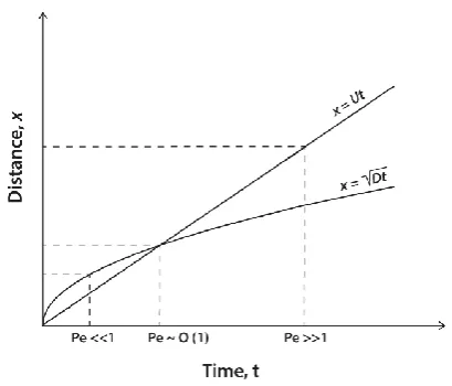
Fig. 1. The relationship between characteristic length,x, and time,
t, scales under varying Peclet number conditions. Under Pe1, advective processes dominate (Regime I); under Pe1 diffusive processes dominate (Regime II); when Pe∼O(1), the characteristic length and timescales are set where the advection and diffusive lines intersect.
individual element. Both timescales provide opportunity for exposure. Averaging of transit and isolation timescales may provide an “effective” exposure timescale, however biogeo-chemical processes are frequently different under connected versus disconnected conditions. If we are aiming to extend the Da approach, it is critical that the relevant biogeochemi-cal processes are identified for each condition and thus tem-poral averaging across conditions may not be appropriate.
The choice of appropriate control volume determines rel-evant time and length scales as well as boundary condi-tions and thus becomes critical for application of our gov-erning equations. An initial assumption is that the control volume and therefore the characteristic length scale,1xi, are
physically constrained, typically by geomorphology (for ex-ample by the catchment, stream or wetland). The sizes of hydrologically isolated systems are by definition physically constrained.
For hydrologically connected systems, the relevant expo-sure timescale, τE, is then determined by the length scale and the transport process (Fig. 1). Note that exposure length scales can be highly variable between individual flow paths and require an appropriate definition of the hydrological problem. In many cases it may be convenient to use a mean length scale for a specific system. When a control volume is not physically constrained, it may be defined operationally, depending on the objectives; an example of this approach is given in Sect. 2.3.
The exposure timescale for hydrologically connected ele-ments under advective conditions is then given as
τEA = 1x
Fig. 2. Regime I: (a) transport and fluxes of chemicalB across hydrologically or hydraulically connected elements are dominated by advection. Examples of this regime are a river under high flow conditions (b), a wetland with groundwater throughflow under a large hydraulic gradient (c) and porous media flow under a large hydraulic gradient (d).
Examples of aquatic systems that are dominated by advective transport are shown in Fig. 2.
The exposure timescale for hydrologically connected ele-ments under diffusive conditions, is given as
τED = 1x
2 i
Deff. (5)
Examples of aquatic systems that are dominated by diffu-sive transport are shown in Fig. 3. We note that exposure timescales may be defined differently by stochastic transport models; any carefully formulated definition may be utilized in the framework.
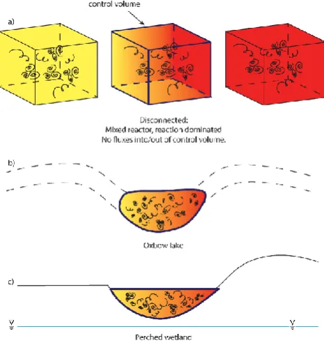
[image:5.595.47.294.62.440.2]When hydrological elements are materially disconnected or isolated, the exposure timescale in the isolated element is equivalent to the isolation timescale, τEI. If the element
Fig. 3. Regime II: (a) transport and fluxes of chemicalB across hydrologically or hydraulically connected elements are dominated by diffusion. Examples of this regime are a river under very low flow conditions, where for example transverse transport exceeds longitudinal transport (b), a wetland at equilibrium with the local groundwater (c) and porous media flow under minimal hydraulic gradient (d).
undergoes periodic connection and disconnection (for ex-ample on an annual basis), τEI is related to the connection or disturbance frequency,kD, a concept used extensively in
We stress again that isolation may be defined both hydro-logically and materially. As commented above, connectivity (and therefore isolation) has previously been defined based on hydrology. When water flows between elements, they are hydrologically connected. When water no longer flows be-tween elements, they are hydrologically isolated. However, if material is consumed or settled prior to reaching the adja-cent element, material isolation of elements is possible even during hydrological connectivity. For material isolation, the efficiency of material transfer will be poor. Our definition of “poor material transfer” is arbitrary and will vary with ap-plication. In some contexts, a 50 % transfer of material be-tween elements may define them as materially isolated. In other applications, 1 % material transfer between elements may define isolation. Examples of aquatic systems that are materially isolated are shown in Fig. 4.
2.2.2 Material processing timescales
Term III in Eq. (2) contains a rate constant for material pro-cessing, such as chemical reaction, seed dispersal and recruit-ment, nutrient uptake, biogeochemical cycling, etc. We con-tinue below with a focus on biogeochemical cycling. While acknowledging that many biogeochemical processes have more complex kinetics, we initially assume our chemical re-action of interest can be described as
A+B −→k C +D. (6) Equation (6) can be treated as a second order reaction where
kis the second order rate constant (m3mmol−1s−1). But if we assumeAto be in excess ofB, then Eq. (6) can be con-sidered “pseudo-first-order” with respect toB, where [B] is not limiting and
d[B]
dt = −k
0[
B], (7)
wherek0is the pseudo-first-order rate constant (s−1) and is used in Eq. (2). The material (in this case chemical) process-ing timescale is then
τP =1/ k0. (8)
For reactions mediated by microbes and enzymes, we can use a Monod kinetic model (Park and Jaffe, 1995; Sch¨afer et al., 1998), which describes the rate of microbial growth as a function of substrate concentration:
d[X]
dt =µmax
[B]
Ks+ [B]
[X], (9)
whereµmax is the maximum specific growth rate (day−1),
[X] is the concentration of cells (cells L−1) andKsis the
sub-strate half-saturation constant (mmol L−1). The correspond-ing equation for the rate of substrate consumption is
d[B]
dt = −qmax
[B]
[image:6.595.311.544.63.311.2]Ks + [B][X] (10)
Fig. 4. Regime III: (a) the elements of interest are hydrologically and hydraulically disconnected. Examples of this regime are an oxbow lake, which has disconnected from its river (b), and a wet-land perched above the groundwater table (c).
where qmax is the maximum specific consumption rate
(mmol cell−1day−1) and
qmax =µmaxY,
whereY is the cell yield (mmol cell−1). We define the
char-acteristic timescale as being the time at which [B] = Ks and
thus
τP = 2
µmax. (11)
Note that processing timescales are intrinsic timescales de-rived from rate laws describing reactions taking place at the scale of the reactants (e.g. microorganisms, microbial con-sortia, biofilms, mineral surfaces) with full access to sub-strate or under conditions of complete mixing. Under con-ditions where short exposure timescales constrain access to substrate and/or reaction, the effective processing timescales may be significantly longer than intrinsic timescales (and hence, under 1st order conditions, effective rate constants will be less that intrinsic rate constants). Careful analysis is required to clarify whether intrinsic or effective processing timescales are desirable or useful to a specific problem; the use of effective processing timescales may remove the signa-ture of key drivers of a system.
2.3 Non-dimensional numbers
the Mach number, the Reynolds number and the hydraulic gradient. Battiato and Tartakovsky (2011) proposed the use of non-dimensional numbers in hydrological upscaling ap-proaches and to provide quantitative measures of the valid-ity of upscaling approximations. We now explore two non-dimensional variables that make up the key components of our connectivity framework.
The non-dimensional Peclet number, Pe, provides the bal-ance between advection and diffusion under hydrological connectivity as
Pe= τ
D E τEA
= ui1xi
Deff
, (12)
where1xiis the characteristic length scale over which
trans-port processes are operating. The Pe is used to determine whether Terms I or II in Eq. (2) are retained.
The Damk¨ohler number (Eq. 1) has been used extensively in chemical engineering and more recently in environmen-tal and hydrological contexts. However, the definition of Da implicitly assumes hydrological or hydraulic connectivity. Without hydrological connectivity, there is no transport of chemicals between hydrological elements, therefore we are unable to defineτT. For example, Da could not be used to characterise hydrologically disconnected systems that are de-fined by the isolation timescaleτEI.
To characterise material fate during both hydrological con-nection and disconcon-nection, we propose the use of the more general form
NE = τE
τP (13)
whereτEis the generalized exposure timescale,τPis a gen-eralized processing timescale, andNEgives an indication of the extent of material processing possible within the expo-sure timescale. For hydrologically connected elements, when
NE1, material is transferred conservatively between
ele-ments; whenNE1, material will have plenty of
opportu-nity to be processed within the exposure times. For a hydro-logically isolated element, whenNE1, material is unlikely
to be processed while that element is isolated; whenNE1,
material will be processed during isolation.
For systems that are intermittently connected, we suggest separate estimation ofNEfor the connected and disconnected conditions. This forces us to define exposure and processing timescales for both conditions, allows assessment of the eco-logical significance of each condition (is the isolated state more significant? or is it the connected state that is important for the system? or both?) and facilitates decisions on appro-priate spatial or temporal averaging of exposure timescales. Even if the isolation timescalethe transport timescale, their relevance for material connectivity depends onNE. If NE1 during isolation, andNE1 during transport, then
the isolation period will be ecologically relevant even if it is shorter than the subsequent transport timescale. A priori av-eraging to obtain an “effective” exposure timescale may in
fact remove critical information about fundamental controls on the ecosystem.
There are times when the length scale of a control volume is not physically constrained, instead the physical dimensions of the control volume may be arbitrarily sized to ensure, for example, that 90 % of material of interest within the control volume is processed. If we take an example of a pseudo-first-order reaction occurring across a hydrologically connected system, and using Eq. (13), then Eq. (7) can be integrated to obtain
[B]∗= [B]0exp −k0τE
= [B]0exp(−NE) (14)
where[B]∗is [B] att=τEand[B]0is [B] att= 0.
When chemicalBis 90 % removed,
[B]∗
[B]0 =0.1=exp(−NE) , (15)
thenNE∼2.3. So for a system whereNE2.3, we expect
more than 90 % removal of chemical. For a system where
NE2.3, we expect less than 90 % removal of chemical. This framework also has application for the definition of ma-terially isolated systems and highlights that material isolation is a function ofNE, rather than an absolute concept.
Examples of the use ofNE for specific contexts are pre-sented below and as case studies in the discussion. The def-inition of boundary and initial conditions are required as the framework is applied, and their magnitude and charac-ter (e.g. constant or varying with time) will depend on ap-plication. This is analogous to the application of the non-dimensional Reynolds number, Re, which describes the bal-ance between inertial and viscous forces and is used to char-acterise environmental flows. Re is defined by the context or application, requiring careful definition of the system, its rel-evant length scales, and thus velocities. These velocities may be estimated via order of magnitude estimates, via experi-mental data or via complex numerical modeling. The scale-dependent Re provides a framework for conceptualizing a problem and provides a degree of generalization across sys-tems. We envisage a similar utility ofNE.
2.4 Special cases
2.4.1 Regime I: advection dominated
For systems that are hydraulically or hydrologically con-nected and Pe1, i.e. the system is advection dominated (Fig. 2), Term II in Eq. (2) drops out, leaving
∂[B]
∂t =ui ∂[B]
∂xi −k 0[B].
I II (16)
Substituting Eq. (4) andk0into Eq. (13) gives
NEA = τE
τP
= k 01x
ux
WhenNE1,τEτP, which indicates that the control vol-ume exposure time is sufficiently long for chemicalsAandB
to react. WhenNE1,τTτP, which indicates that chem-icalsAandBdo not have sufficient time to react before they are advected out of the control volume; in this case chemi-calsAandBmay be treated as if they are conservative.
In the large Pe limit, the general solution Eq. (3) can be re-written as
[B] =exp(−k0t ) f (x−uxt ) (18)
where the functionf (x)represents the initial (t= 0) distri-bution of [B] in the element. As time increases, the initial profile of [B] is advected at speedux between the elements
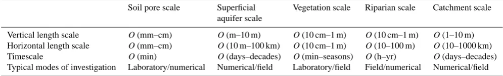
with a reduction in magnitude due to the reaction term. This solution and its behaviour are shown in Fig. 5a and b. Figure 5a shows the case where there is no significant con-sumption ofB(NE1) before it has been advected between
the elements. The magnitude of the initial profile has been preserved. Figure 5b shows a reduction in the magnitude of the profile due to significant consumption of B (NE1). Note, however, that B has not spread during transport be-tween the elements since this is the advection-dominated regime (i.e. diffusion is minimal).
2.4.2 Regime II: diffusion dominated
For systems that are hydraulically or hydrologically con-nected and Pe1 (i.e. system is diffusion dominated, Fig. 3), Term I in Eq. (2) drops out; so we have
∂[B]
∂t =Deff ∂2[B]
∂xi∂xi −k 0[B],
II III (19)
and given Eq. (5), then
NED = k 01x2 Deff
. (20)
When Pe1, the general solution Eq. (3) can be re-written as
[B] =exp(−k0t )
"
α0+ ∞ X
n=0
αncos n π
1xi x
+βnsin n π
1xi x
exp −n
2π2D eff 1xi2 t
!#
. (21) In the absence of significant reaction (NE1),Bwill even-tually diffuse through the entire system without significant loss ofB. This is shown in Fig. 5c. Alternatively, ifNE1,
then much ofB will be used up before it has a chance to diffuse through the system, which is shown in Fig. 5d.
[image:8.595.310.547.61.266.2]The idealized solutions discussed above for Regimes I and II have assumed some initial distribution of [B] and pe-riodic boundary conditions. More general boundary condi-tions (for example fixed flux or fixed concentration boundary
Fig. 5. Example profiles of [B] from the model problem for small (solid line) and large (dashed line) times illustrating the evolution of [B] under different conditions: (a) Pe1 and NE1, (b) Pe1 and NE1, (c) Pe1 and NE1, (d) Pe1 and NE 1. Note that in this figure,B and xhave been normalized for illustrative purposes.
conditions) do not affect the general framework and regimes outlined above. The fate of inflows at the boundaries of the element is determined by the element’s regime.
2.4.3 Regime I and II boundary
We have shown how to use Pe andNEto characterise
hydro-logical systems, however porous media are frequently char-acterised by their dispersivity,
αi = Deff
ui
. (22)
If we normalize the dispersivity by the characteristic length scale (i.e. the length of the control volume), then
αi 1xi
= Deff
ui1xi
= 1
Pe. (23)
Note that this relationship is dependent on scale and the em-pirically derived relationship
αi =0.01751xi1.46 (24)
can be applied to a flow path length less than 3500 m (Todd and Mays, 2005).
condition, advection and diffusion act on similar timescales and either Eq. (17) or Eq. (20) can be used.
It has been demonstrated that in porous media, when
Pe∼O(1), the progress of a reaction can be limited by in-complete mixing of flow paths containing the different reac-tants (e.g. O2and Fe(II)) (Cirpka and Attinger, 2003).
Incom-plete mixing results in a reduced exposure timescale (which is a function of the mixing frequency) and therefore the effec-tiveness of a reaction (or process) is diminished even though the processing timescale may be quite short or even instanta-neous (Gramling et al., 2002). This highlights the need to ac-curately determine exposure timescales and the caution with which we should utilize spatially or temporally averaged ex-posure timescales.
2.4.4 Regime III – hydrological disconnection
When hydrological elements become hydrologically isolated with no water fluxes in or out, the chemical reaction shown in Eq. (6) may quickly become limited, by either the depletion of reactants or the build up of products. The consequences of hydrological/hydraulic isolation are no resupply of reac-tants and no flushing of products. Under these conditions, the change in concentration ofBcannot be described by Eq. (7), however to illustrate our conceptual framework we will as-sume that until chemicalB is 10 % consumed, pseudo-first order kinetics can be utilized, i.e. the reaction is not limited by [A]. In this case we revert to using
∂[B]
∂t = −k
0[
B]. (25)
The general solution Eq. (3) can then be re-written simply as
[B]t =B0exp(−k0t ) (26)
where[B]0 is the spatially averaged concentration of B at
t= 0, and then
NEI =τIk0. (27)
3 Discussion
3.1 Application ofNEapproach across scales
In the previous sections we outlined how NE and Pe can be used to characterise hydrological systems according to the fate of chemicalB. We will now examine this concept across different temporal and spatial scales. We will focus on the oxidation of Fe(II), which plays a prominent role in linking metabolic activities across anaerobic and aero-bic components of aquatic systems (Raiswell and Canfield, 2012). Fe(II) oxidation is an ecologically significant reaction both under neutral and acidic conditions, however the rate is strongly dependent on pH (Stumm and Morgan, 1996).
The oxidation process typically implies precipitation of fer-ric oxides and through that the generation of acidity. Un-der well-buffered conditions, such as anaerobic ground or pore waters, the pH remains relatively constant. Under low or no-alkalinity conditions however, oxidation of Fe(II) sig-nificantly contributes to acidification of surface waters. Ex-amples of such systems are acidic mining lakes (Peine et al., 2000) or acid sulphate soils (Burton et al., 2006) where acid-ity has been generated through the oxidation of pyrite, but where acidic iron cycling, i.e. the combined reduction of fer-ric and oxidation of ferrous iron, maintains acidic conditions (Peine et al., 2000). Here we will compare anaerobic aquatic systems containing Fe(II) and how they respond to oxygen exposure under different transport regimes. We have cho-sen two pH conditions: neutral (pH 7) conditions as found in many anaerobic environments, and slightly acidic (pH 4) conditions as found in many anaerobic systems receiving waters that have been exposed to pyrite oxidation (Blodau, 2006).
The oxidation of Fe(II) can be modelled using the rate law given by Stumm and Lee (1961).
d[Fe(II)]
dt = −kabioPO2
OH−2[Fe(II)] (28) where PO2 is the partial pressure of oxygen (0.21 atm) and kabio is the abiotic rate constant (1.5×10¹³L2mol−2 atm−1min−1at 25◦C).
This rate law predicts extremely low oxidation rates under acidic conditions. Typically, Fe(II) oxidation will be accel-erated by bacteria. Pesic et al. (1989) reported a decrease in microbial oxidation rate with increasing pH between pH 2.2 and pH 3. Extrapolation of their rate law (Kirby et al., 1999) demonstrates that at pH 4 the abiotic rate is still higher then the microbial rate. Hence, in our examination we will use Eq. (28) for pH 4 and pH 7. The rate constantkin Eq. (28) can be converted into a pseudo 1st-order rate constant for ambient temperature and pressure conditions, and for a pre-defined pH, as
k0 =kabioPO2
OH−2 (29)
wherek0yields the reaction times,τR=τP (Table 2), which will be used for the analyses below.
3.1.1 Case I: porewater transport in deep lake sediments
The sediment of deep eutrophic lakes (pH neutral con-ditions) or mining lakes (acidic concon-ditions) may be hy-drologically connected to the surrounding groundwater, but if the hydraulic conductivity of the sediment material is extremely low, groundwater inflow velocities could be
<10−9m s−1. We assume a molecular diffusion coefficient,
Deffof 10−9m2s−1.
Table 2. Pseudo-first order rate constants,k0, and processing (reac-tion) timescales,τP, for the oxidation of iron(II) under different pH conditions.
pH k0(min−1) τP(s)
7 3×10⁻² 2×10³ 4 3×10⁻⁸ 2×10⁹
which the O2concentration has been decreased to a specified
level. In order to fulfil the validity of pseudo-first order kinet-ics, we assume a reduction by only 10 %, i.e.1PO2= 0.021 atm which corresponds to1[O2] ≈0.03 mmol L−1at
ambi-ent temperature, and stoichiometrically that corresponds to an Fe(II) consumption of 1[FeII] = 0.03 mmol L−1. Hence, the thickness of a layer will be estimated, in which the oxy-gen concentration does not drop below 0.27 mmol L−1.
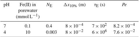
Fe(II) concentrations in pH neutral lake sediments rarely exceed 0.1 mmol L−1 (see e.g. Baccini, 1985; Gelhar et al., 1992), while in acidic environments Fe(II) concentrations of up to 10 mmol L−1may be reached (Burton et al., 2006; Peine et al., 2000). Therefore, a1[FeII] of 0.03 mmol L−1is a 30 % removal at pH 7 and a 0.3 % removal at pH 4. Using Eq. (15),NE≈0.4 and 0.003 for pH 7 and 4, respectively.
In the next step we can estimate 1x10% by combining Eqs. (5) and (20) as
1x10% = q
NED·τP ·Deff, (30) which yields 8×10⁻⁴m at pH 7, and 8×10⁻²m at pH 4. The corresponding exposure timescales, τED, within these contact zones are 7×10²s at pH 7, and 6×10⁶s at pH 4. Using these length scales, a groundwater inflow velocity of 10−9m s−1 and the molecular diffusion coefficient, Pe, ranges from 8.2×10⁻⁴at pH 7, to 7.6×10⁻²at pH 4 (Ta-ble 3), which indicates diffusive conditions and supports ap-plication of Eq. (5).
The above calculations have two specific implications. Firstly, the thickness of the layer that remains close to O2
sat-uration varies significantly between the two pH regimes. The zone of Fe(II) production from dissimilatory iron reduction (a biogeochemical process sensitive to O2) will be shifted
to deeper sediments under acidic conditions. Secondly and more importantly, the timescale of exposure to oxygen satu-ration is 4 orders of magnitudes longer under acidic condi-tions and lasts for several weeks. Note that the calculatedτE
is a lower estimate and may be even longer at lower Fe(II) concentrations. This long timescale provides ample opportu-nities for interference from other biogeochemical processes that involve oxygen or consume Fe(II).
Hence,NEcan be regarded as a process-specific
parame-ter that allows us to characparame-terise hydrological systems based on chemical fate. When NE∼O(1), as was calculated
un-der pH 7, the balance between exposure and processing is
Table 3. Estimates of relevant parameters and non-dimensional numbers at pH 4 and 7.
pH Fe(II) in NE 1x10%(m) τE(s) Pe porewater
(mmol L−1)
7 0.1 0.4 8×10⁻⁴ 7×10² 8.2×10⁻⁴ 4 10 0.003 8×10⁻² 6×10⁶ 7.6×10⁻²
critical and the system will be sensitive to shifts in hydro-logical regime. WhenNEO(1), as was calculated under
pH 4, the system will not be sensitive to shifts in hydrologi-cal regime.
3.1.2 Case II: Surface water – groundwater exchange
The advective recharge of oxygenated surface waters into Fe(II)-rich groundwater is very common in many riparian systems under losing conditions. While the majority of these systems are pH neutral, wetlands affected by acid sulphate soils (Johnston et al., 2011) and mining lakes (Fleckenstein et al., 2009) may lose acidic water to groundwater.
Again under this scenario, the characteristic length scale is not physically constrained, and we can again estimate the length scales over which the O2concentration has been
de-creased by 10 %. The Fe(II) boundary conditions are selected as in Case I.1x10% can now be calculated using Eqs. (4) and (17) as
1x10% =uxτPNEA (31)
whereuxis set to 10−5m s−1for this scenario.
The distance from the riparian zone over which 10 % of O2is consumed is 6.8×10⁻³m at pH 7, and 5.7×101m at
pH 4. In other words, after 57 m of flow across a riparian zone at pH 4 the system would still be close to oxygen saturation, allowing O2consuming reactions.
To calculate Pe numbers for Case II, we can use Eq. (23). In porous-media flow,Deff becomes a scale-dependent
persion coefficient, which can be estimated from the dis-persivity, α, of the aquifer into which the lake water penetrates (see Eqs. 22 and 24). We get αi= 1×10⁻⁵m
and Deff= 1×10⁻¹⁰m2s−1 for pH 7, and αi= 6.4 m and
Deff= 6×10⁻⁵m2s−1 for pH 4. Thus at pH 7, i.e. within the short distance of 6 mm, no dispersion occurs. The corre-sponding Pe ranges from 5.7 ×10²at pH 7 (indicating ad-vective transport through the O2containing layer) to 8.9 at
pH 4 (indicating advective transport with contributions from dispersive mixing).
[image:10.595.110.224.106.151.2]conditions (and how they vary with time), we could size the riparian width to the length scale,1x, that is required to re-move, for instance, 90 % of the nitrate that has infiltrated to groundwater from agricultural land. To some extent the “50-day line” typically applied to constrain drinking water zones implicitly uses this concept already.
3.1.3 Case III: temporarily disconnected systems
Floodplain wetlands and playas frequently become temporar-ily disconnected from surface and sub-surface water flow pathways. In Western Australia, shallow groundwater-fed wetlands affected by acid sulphate soils fill with Fe(II)-rich groundwater, which is then exposed to O2(Nath et al., 2013).
Seasonal lowering of the groundwater table disconnects the wetlands from the source of Fe(II), and its subsequent oxida-tion via ongoing exposure to O2is controlled by the isolation
timescale, i.e.τEI. Depending on the buffering capacity of the wetland mineralogy, both acidic and neutral conditions can be observed.
Under this scenario, the characteristic length and timescales are physically constrained. If we assume a typi-calτEI∼100 days (∼107s), then using Eq. (14), we estimate the extent of Fe(II) oxidation as 100 % at pH 7 and 1 % at pH 4. The differences between Fe(II) oxidation at the differ-ent pHs can also be demonstrated byNE. Using Eq. (13),NE
is 5×10³ at pH 7 (indicating the disconnection timescale provides sufficient exposure opportunity for the reaction to proceed) and 5×10⁻³at pH 4 (indicating that the disconnec-tion timescale does not provide enough time for the reacdisconnec-tion to proceed). Of course these calculations assume the wetland waters are fully mixing at all times. Any density stratification within the wetland will reduceτEI, i.e. the timescales over which Fe(II)-rich bottom waters are exposed to O2-rich
sur-face waters. Density stratification may also alter the control volume utilized and therefore the spatial averaging of chem-ical concentrations.
3.2 Competiveness of reactions
We have shown thatNE numbers are reaction specific; the corresponding spatial scales are also reaction dependent and not always controlled by geomorphology. In a first approach, we can therefore argue that lowNEfor a certain reaction im-plies ample opportunity for alternative reaction pathways to proceed between materially connected elements or within a materially isolated element. Inversely, highNEimplies pre-dominance of the biogeochemical process of interest.NE
al-lows us to compare the effectiveness of different material processing reactions across a certain temporal (τE) or spatial
(1x) scale.
More generally, lowerNEimplies lower competiveness of
a specific reaction. In the examples discussed above, the ox-idation of Fe(II) is much more competitive at pH 7 than at pH 4. In this case competiveness is clearly controlled by the
large differences ink0. However,NEis of course also affected by the exposure timescale. We therefore propose that for a given system,NEcan be used as a general parameter to com-pare competiveness between different reactions of interest.
Competiveness of redox reactions is typically discussed in terms of thermodynamic arguments, for example the gain in free energy,1Gf, obtained from oxidation of organic matter
(Zehnder and Stumm, 1988). This concept works very well in diffusion controlled systems such as the sediment porewaters of the ocean or deep lakes. Attempts to adapt this concept to groundwater systems have been problematic. Rather, zones of intensive redox activity are observed to be spatially dis-tributed or located at plume fringes (see e.g. Prommer et al., 2006). Considering that the rate of a reaction is proportional to 1Gf, thermodynamics are also related to the reaction timescale. Considering further that all dissolved substances have appropriately the same diffusion coefficients and that their residence times under diffusion controlled conditions are approximately identical, then it becomes clear that1Gf
andNE are interrelated predictors for competiveness under
diffusion-controlled (or well-mixed) conditions.
Under advection or dispersion controlled conditions, how-ever, the timescale of exposure along a flow path varies strongly depending on external forcing. Of course the flow paths and therefore exposure timescales may be distributed in space, similar to residence times, and this spatial vari-ability will give rise to a patchwork ofNE values, parallel-ing the concept of “residence time distributions” with each controlled by specific biogeochemical regimes. Under these conditions, chemical competiveness becomes dependent on the ratio of processing/reaction to exposure timescales;NE
therefore can be used as a general parameter to compare com-petiveness under all regimes.
3.3 Intermittent connectivity and ecological consequences
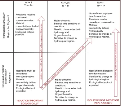
Hydrological systems transition between the regimes out-lined above, according to external forcing. Of particular rel-evance may be shifts between Regime I and II or intermit-tent transition from Regime III, i.e. the disconnected state, to Regime I or II. Estimates ofNEfor the different regimes provide a framework for predicting the biogeochemical and ecological significance of the shifts (Table 4).
1144 C. E. Oldham et al.: A generalized Damk¨ohler number for classifying material processing
Table 4. A summary of system characteristics under the different regimes and as a function ofNE. Note that once elements become connected after a period of isolation, it is possible for them to rapidly move across regimes. The balance between exposure timescales (both connected and isolated) and processing timescales determines the ecological signficance of the period of isolation and the regime shift.
39
function of NE. Note that once elements become connected after a period of isolation,
799
it is possible for them to rapidly move across regimes. The balance between
800
exposure timescales (both connected and isolated) and processing timescales
801
determines the ecological signficance of the period of isolation and the Regime shift.
802
803
804
805
NE>> 1 TE>> TP
NE<< 1 TE<< TP NE ~O(1)
TE ~ TP
Regime I or Regime II
Re
gime III
Not sufficient exposure time for reaction. Reactants can be considered conservative. Material
connectivity defined hydrologically. Sensitive to change in hydrological regime. Highly dynamic.
Balance very senstiive to conditions.
Need to characterise both hydrology and
biogeochemistry. Sensitive to change in hydrological regime.
Reactants must be considered non-conservative. Material
connectivity defined biogeochemically. Ecological hotspot expected.
Highly dynamic. Balance very senstiive to conditions.
Need to characterise both hydrology and
biogeochemistry. Sensitive to change in hydrological regime.
Not sufficient exposure time for reaction. Sensitive to change in hydrological regime. Ecological hotspot not expected.
ISOLATION IMPORTANT ECOLOGICALLY
ISOLATION NOT IMPORTANT ECOLOGICALLY Reactants must be
considered non-conservative. Material
connectivity controlled biogeochemically.
possible Ecological hotspot
Hydrological l connectivity
H
ydr
olog
ical or ma
ter
ial
disc
onnec
tivit
y
Effec tive ma
terial tr ansfer, isola
tion impor tant ec
olog ically
Limit
ed ma
ter
ial tr
anf
er possivle within e
xposur
e timescale
Connec
tivit
y less impor
tan
t ec
olog
ically
The magnitude of such pulses typically depends strongly on the antecedent conditions (e.g. Inamdar et al., 2004). Knorr (2013) observed that Fe and DOC were exported to streams during rainfall events only if the preceding period allowed a pool of Fe and DOC to be created (Regime I). In-versely, after a rainfall event, a rapid transfer of Fe to the stream would require the prevention of oxidation and reten-tion at the site (Regime II). If we apply theNEframework to
this example, we can see that if the Regime I (pre-event)NE
for the formation of Fe(II) is high, a large pool of dissolved Fe can build up. In contrast, effective transfer of Fe into the receiving stream during a rainfall event requires the Fe(II) oxidation timescale to be longer than the (typically short) exposure timescale, i.e.NE<1. As in our case studies, the oxidation timescale depends strongly on pH. The oxidation kinetics may also be dependent on DOC-Fe(II) complexation which stabilizes Fe(III) as colloids and thus promotes export of Fe associated with DOC (Llang et al., 1993). During peri-ods of shifting exposure times, changes inNEusefully high-light the different controls on material connectivity across a
hydrological system and its impact on material transfer out of the system.
An interesting example for our discussion of material con-nectivity is given by Basu et al. (2011b) in an exploration of hydrological versus biogeochemical controls on the catch-ment scale, which can be reanalysed usingNEnumbers. Basu
surface waters, and the transfer rate fluctuates with the size of the accumulated pool. For such episodic events,NE1 during time of disconnection in the soil surface, andNE1 at the catchment scale, allowing detection of the substance during subsequent connection.
Gradients ofNE in either space or time may also be
in-dicative of sinks or sources. When NE for a specific
pro-cess and a specific hydrological element is large relative to it neighbouring elements, a concentration gradient may be established and a “hotspot” of material processing formed. WhenNEfor an element is large relative to the preceding or subsequent conditions, a “hot moment” may form. We sug-gest that it is the shift inNE that is critical for hot spot or hot moment formation, rather than a regime shift. Some of the possible ecological consequences of shifts inNEare ex-plored in Table 4.
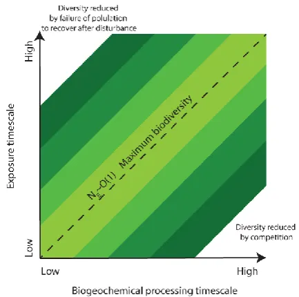
[image:13.595.317.534.60.275.2]So far we have constrained ourselves to considering spe-cific biogeochemical reactions occurring within elements of the hydrological cycle. Finally, we broaden our focus to con-sider landscape-scale ecological processes and their charac-teristic timescales. The extent to which an ecosystem is re-silient to environmental perturbations is likely controlled by the relative rates at which a biological community can re-spond to environmental change or disturbance (i.e.k0) and the exposure timescale of the relevant element. If we set the biogeochemical rate, k0, to be analogous to population growth rate and the exposure timescale,τE, to be analogous to exogenous timescales (Hastings, 2010) or the reciprocal of the disturbance frequency, then our two timescales have direct analogues to concepts in terrestrial ecology. For ex-ample, Huston (1994) suggested that the ratio of the popula-tion growth rate to the disturbance frequency, i.e.NEin our framework, impacts on biodiversity and ecological resilience (Fig. 6).
Of particular interest is the conceptual understanding that community biodiversity is maximal when there is a balance between population growth rate (or biogeochem-ical reaction rate) and disturbance frequency, i.e. when
NE∼O(1) (Huston, 1994, Fig. 6). The biodiversity in turn
affects ecosystem resilience (Gunderson, 2000; Scheffer and Carpenter, 2003); however, the stability space within which ecosystem resilience operates is determined by external fac-tors, and has been related to characteristic spatial or tempo-ral scales of external forcing (Scheffer and Carpenter, 2003). We have shown above that NE is process-specific so the question arises whether we can describe the resilience of a system in terms of itsNEdistribution. This requires further investigation.
Fig. 6. The relationship betweenNEand biodiversity. This is likely to hold true for microbial diversity as well as landscape-scale bio-diversity. Modified from Huston (1994).
4 Conclusions
The concepts discussed above provide a general and holis-tic framework to analyse and characterise system behaviour in terms of the effectiveness of material processing, defined by the non-dimensional numberNE, as the ratio of the expo-sure timescale to the material processing timescale. The use of this framework has multiple benefits: (a) it focuses our at-tention on clearly defining our system, its spatial scales and the material processing (or reaction) of interest; (b) it high-lights that “transport limitation” is a relative concept and de-pends on the material processing of interest; (c) it allows us to incorporate isolated systems within a hydrological systems understanding; (d) it provides insights into the likely ecolog-ical significance of shifts in hydrologecolog-ical forcing; (e) it can be used for clarification of whether the balance in control-ling mechanisms is constant with scale-up; (f) it can be used for water management as it allows us to appropriately size water remediation options; and (g) it can be used in the de-sign of monitoring programs to ensure that monitoring scales capture the key dynamics of a system.
TheNEframework is simple in definition but challenging to apply. Identification of appropriate exposure and process-ing timescales for the system of interest is not trivial. Appli-cation of theNEframework requires a clear definition of the
problem and a sound rationale for the choice of timescales and the methods used for their determination. These meth-ods can range from numerical simulations to geochemical or isotopic analysis. TheNEframework certainly helps to
Appendix A
Notation.
Variable Units Description
αi m Dispersivity ini-direction
αn dimensionless Fourier cosine coefficient
βn dimensionless Fourier sine coefficient
[B] mmol L−1 Concentration of chemicalB
[B]max mmol L−1 Maximum expected concentration of chemicalB [B]0 mmol L−1 Initial concentration of chemicalB
Da dimensionless Damk¨ohler number
Deff m2day−1 Effective diffusion coefficient
k0 s−1 First order rate constant
kabio L2mol−2atm−1min−1 Abiotic rate constant for iron oxidation
n dimensionless Summation index
NE dimensionless Ratio of exposure to processing timescales
NEA dimensionless Ratio of exposure to processing timescales (advective regime)
NED dimensionless Ratio of exposure to processing timescales (diffusive regime)
NEI dimensionless Ratio of exposure to processing timescales (isolated regime)
Pe dimensionless Peclet number
PO2 atm Partial pressure of oxygen qmax mmol L−1day−1
t unit of time Time
τT unit of time Transport timescale
τR unit of time Reaction timescale
τEA unit of time Characteristic exposure timescale (asdvective regime)
τED unit of time Characteristic exposure timescale (diffusive regime)
τEI unit of time Characteristic exposure timescale (isolated regime)
τP unit of time Characteristic processing timescale
ui m day−1 Velocity ini-direction
ux m day−1 Velocity inx-direction
xi m Distance ini-direction
1x m Characteristic length scale inx-direction
1x10% m Characteristic length scale required for 10 % of reactant to be removed
community, protocols for the delineation of timescales will develop.
This work has opened up an array of questions but per-haps the most intriguing question is how we most effectively analyse intermittently disconnected systems. Is it preferrable to take a stochastic approach, using an ensemble of exposure timescales? The parameter analysed could vary depending on assessed ecological significance, but could involve (a) the isolation timescales, (b) the connection timescales, and/or (c) the ratio of the isolation to connection timescales.
We expect that in many systems there will also be an en-semble of reaction timescales, so a pdf would also be re-quired. We also expect the exposure timescales to have sig-nificantly greater variance than the reaction timescales. The ratio of these two pdfs would create anNEpdf, which would
in turn characterise material connectivity between systems. A full exploration of the stochastic nature ofNE is needed
and requires analysis of multiple exemplar data sets.
Acknowledgements. The authors would like to express thanks to
a large number of people who over the years have contributed to lively discussion on the use of Da and other non-dimensionless numbers for characterising catchments, including Carlos Ocampo, Murugesu Sivapalan, Jeff McDonnell, Paul Lavery, Ursula Salmon and Wolfgang Kurtz. This collaboration was supported by DFG grant Pe 438/20-1.
Edited by: S. Thompson
References
Ali, G. A. and Roy, A. G.: Shopping for hydrologically representative connectivity metrics in a humid temper-ate forested catchment, Wtemper-ater Resour. Res., 46, 1–24, doi:10.1029/2010WR009442, 2010.
Baccini, P.: Phosphate interactions at the sediment-water interface, in: Chemical Processes in Lakes, edited by: Stumm, W., Wiley Online Library, 1985.
Basu, N. B., Rao, P. S. C., Thompson, S. E., Loukinova, N. V., Don-ner, S. D., Ye, S., and Sivapalan, M.: Spatiotemporal averaging of in-stream solute removal dynamics, Water Resour. Res., 47, W00J06, doi:10.1029/2010WR010196, 2011a.
Basu, N. B., Thompson, S. E., and Rao, P. S. C.: Hydrologic and biogeochemical functioning of intensively managed catch-ments: A synthesis of top-down analyses, Water Resour. Res., 47, W00J15, doi:10.1029/2011WR010800, 2011b.
Battiato, I. and Tartakovsky, D. M.: Applicability regimes for macroscopic models of reactive transport in porous media, J. Contam. Hydrol., 120-121, 18–26, doi:10.1016/j.jconhyd.2010.05.005, 2011.
Beven, K. J.: Rainfall-runoff modelling: The primer, Wiley, New York, 2001.
Blodau, C.: A review of acidity generation and consumption in acidic coal mine lakes and their watersheds, Sci. Total Environ., 369, 307–332, 2006.
Bolster, D., de Anna, P., Benson, D. A., and Tartakovsky, A. M.: Incomplete mixing and reactions with fractional dispersion, Adv. Water Resour., 37, 86–93, doi:10.1016/j.advwatres.2011.11.005, 2012.
Botter, G., Bertuzzo, E., and Rinaldo, A.: Transport in the hydro-logic response: Travel time distributions, soil moisture dynam-ics, and the old water paradox, Water Resour. Res., 46, 1–18, doi:10.1029/2009WR008371, 2010.
Botter, G., Bertuzzo, E., and Rinaldo, A.: Catchment residence and travel time distributions: The master equation, Geophys. Res. Lett., 38, 1–6, doi:10.1029/2011GL047666, 2011.
Burton, E., Bush, R., and Sullivan, L.: Sedimentary iron geochem-istry in acidic waterways associated with coastal lowland acid sulfate soils, Geochim. Cosmochim. Acta, 79, 5455–5468, 2006. Carleton, J. N.: Damkohler number distributions and constituent
re-moval in treatment wetlands, Ecol. Eng., 19, 233–248, 2002. Cirpka, O. A. and Attinger, S.: Effective dispersion in
heteroge-neous media under random transient flow conditions, Water Re-sour. Res., 39, 1–15, doi:10.1029/2002WR001931, 2003. Dankwerts, P. V.: Absorption by simultaneous diffusion and
chemi-cal reaction into particles of various shapes and into falling drops, Trans. Faraday Soc., 47, 1014–1023, 1951.
Detty, J. M. and McGuire, K. J.: Topographic controls on shallow groundwater dynamics: implications of hydrologic connectivity between hillslopes and riparian zones in a till mantled catchment, Hydrol. Process., 24, 2222–2236, doi:10.1002/hyp.7656, 2010. Dooge, J. C. I.: Looking for hydrologic laws, Water Resour. Res.,
22, 46–58, 1986.
Fleckenstein, J., Neumann, C., Volze, N., and Beer, J.: Raumzeit-muster des Grundwasser-Seeaustausches in einem Tagebaurest-see, Grundwasser, 14, 207–217, 2009.
Gelhar, L. W. L., Welty, C., and Rehfeldt, K. R. K.: A critical review of data on field-scale dispersion in aquifers, Water Resour. Res., 28, 1955–1974, 1992.
Gramling, C. M., Harvey, C. F., and Meigs, L. C.: Reactive transport in porous media: a comparison of model prediction with labora-tory visualization, Environ. Sci. Technol., 36, 2508–2514, 2002. Gunderson, L. H.: Ecological resilience – in theory and application,
Annu. Rev. Ecol. Syst., 31, 425–439, 2000.
Hastings, A.: Timescales, dynamics and ecological understanding, Ecology, 91, 3471–3480, 2010.
Hornberger, G. M., Scanlon, T. M., and Raffensperger, J. P.: Mod-elling transport of dissolved silica in a forested headwater catch-ment: the effect of hydrological and chemical time scales on hys-teresis in the concentration-discharge relationship, Hydrol. Pro-cess., 15, 2029–2038, doi:10.1002/hyp.254, 2001.
Hrachowitz, M., Soulsby, C., Tetzlaff, D., Malcolm, I. A., and Schoups, G.: Gamma distribution models for transit time esti-mation in catchments: Physical interpretation of parameters and implications for time-variant transit time assessment, Water Re-sour. Res., 46, doi:10.1029/2010WR009148, 2010.
Huston, M. A.: Biological diversity: The coexistence of species on changing landscapes, Cambridge University Press, Cambridge, 1994.
Inamdar, S. P., Christopher, S. F., and Mitchell, M. J.: Export mech-anisms for dissolved organic carbon and nitrate during summer storm events in a glaciated forested catchment in New York, USA, Hydrol. Process., 18, 2651–2661, doi:10.1002/hyp.5572, 2004.
Johnston, S., Keene, A., Bush, R., Sullivan, L., and Wong, V.: Tidally driven water column hydro-geochemistry in a remediat-ing acidic wetland, J. Hydrol., 409, 128–139, 2011.
Kirby, C., Thomas, H., Southam, G., and Donald, R.: Relative con-tributions of abiotic and biological factors in Fe(II) oxidation in mine drainage, Appl. Geochem., 14, 511–530, 1999.
Klein, C., Wilson, K., Watts, M., Stein, J., Berry, S., Carwardine, J., Smith, M. S., Mackey, B., and Possingham, H.: Incorporat-ing ecological and evolutionary processes into continental-scale conservation planning, Ecol. Appl., 19, 206–217, 2009. Knorr, K.-H.: DOC-dynamics in a small headwater catchment as
driven by redox fluctuations and hydrological flow paths – are DOC exports mediated by iron reduction/oxidation cycles?, Bio-geosciences, 10, 891–904, doi:10.5194/bg-10-891-2013, 2013. Kurtz, W., and Peiffer, S.: The role of transport in aquatic redox
chemistry, in: Aquatic Redox Chemistry, edited by: Tratnyek,P. G., Grundl, T. J., and Haderlein, S. B., American Chemical So-ciety, Washington DC, USA, 559–580, 2011.
Llang, L., McNabb, J. A., Paulk, J. M., Guy, B., and McCarthy, J. F.: Kinetics of Fe(I1) oxygenation at low partial pressure of oxygen in the presence of natural organic matter, Environ. Sci. Technol., 27, 1864–1870, 1993.
McDonnell, J., McGuire, K., Aggarwal, P., Beven, K., Biondi, D., Destouni, G., Dunn, S., James, A., Kirchner, J., Kraft, P., Lyon, S., Maloszewski, P., Newman, B., Pfister, L., Rinaldo, A., Rodhe, A., Sayama, T., Seibert, J., Solomon, K., Soulsby, C., Stew-art, M., Tetzlaff, D., Tobin, C., Troch, P., Weiler, M., West-ern, A., W¨orman, A., and Wrede, S.: How old is streamwa-ter? Open questions in catchment transit time conceptualiza-tion, modelling and analysis, Hydrol. Process., 24, 1745–1754, doi:10.1002/hyp.7796, 2010.
McDonnell, J., Sivapalan, M., Vach´e, K., Dunn, S., Grant, G., Hag-gerty, R., Hinz, C., Hooper, R., Kirchner, J., Roderick, M., Selker, J., and Weiler, M.: Moving beyond heterogeneity and process complexity: A new vision for watershed hydrology, Water Re-sour. Res., 43, 1–6, doi:10.1029/2006WR005467, 2007. McGuire, K. and McDonnell, J.: A review and evaluation of

![Fig. 5. Example profiles of [that in this figure,and NE(solid line) and large (dashed line) times illustrating the evolution of[B] from the model problem for smallB] under different conditions: (a) Pe ≫ 1 and NE ≪ 1, (b) Pe ≫ 1 ≫ 1, (c) Pe ≪ 1 and NE ≪ 1, (d](https://thumb-us.123doks.com/thumbv2/123dok_us/9260549.994995/8.595.310.547.61.266/example-proles-gure-illustrating-evolution-problem-different-conditions.webp)