www.hydrol-earth-syst-sci.net/18/1225/2014/ doi:10.5194/hess-18-1225-2014
© Author(s) 2014. CC Attribution 3.0 License.
Hydrology and
Earth System
Sciences
Challenges in modelling river flow and ice regime on the
Ningxia–Inner Mongolia reach of the Yellow River, China
C. Fu1, I. Popescu2, C. Wang2,4, A. E. Mynett2,3, and F. Zhang5
1NARI Group Corporation, water conservancy and hydropower technology branch company, Nanjing 211000, China 2UNESCO-IHE, Institute for Water Education, 2601DA, Delft, the Netherlands
3Delft University of Technology, Faculty of CiTG, 2600GA, Delft, the Netherlands 4Hydrology Bureau, Yellow River Conservancy Commission, Zhengzhou 450004, China 5Yellow River Institute of Hydraulic Research, Zhengzhou 450003, China
Correspondence to: I. Popescu ([email protected])
Received: 22 July 2013 – Published in Hydrol. Earth Syst. Sci. Discuss.: 11 October 2013 Revised: 31 January 2014 – Accepted: 18 February 2014 – Published: 28 March 2014
Abstract. During winter the Yellow River in China is
fre-quently subjected to ice flood disasters. Possible dike break-ing due to ice floods poses a serious threat to the part of the region located along the river, in particular the Ning– Meng reach (including Ningxia Hui and the Inner Mongolia autonomous regions). Due to its special geographical loca-tion and river flow direcloca-tion, the ice dams and jams lead to dike breaking and overtopping on the embankment, which has resulted in huge casualties and property losses through-out history. Therefore, there is a growing need to develop capability in forecasting and analysing river ice floods. Re-search into ice floods along the river is taking place at the Yellow River Conservancy Commission (YRCC). A numeri-cal model is one of the essential parts of the current research going on at the YRCC, which can be used to supplement the inadequacies in the field and lab studies which are being car-ried out to help understand the physical processes of river ice on the Yellow River. Based on the available data about the Ning–Meng reach of the Yellow River, the YRCC river ice dynamic model (YRIDM) has been tested for capabilities to conduct ice flood forecasting. The YRIDM can be applied to simulate water level, discharge, water temperature, and ice cover thickness under unsteady-state conditions. Differ-ent scenarios were designed to explore the model uncertainty for two bounds (5 and 95 %) and probability distribution. The YRIDM is an unsteady-state flow model that can show the basic regular pattern of ice floods; hence it can be used as an important tool to support decision making. The recommen-dation is that data and research should be continued in order to support the model and to measure improvements.
1 Introduction
River ice is a natural phenomenon that can be commonly seen in the cold regions of the world. River ice plays an im-portant role in cold regions, being the main transportation means in wintertime: the ice roads and ice bridges caused by river ice in the northern regions of Canada, Russia, and the USA (Alaska), where the population is sparse, are a pos-itive effect of the ice formation in cold regions (Petrow et al., 2007; Rojas et al., 2011). However, on the negative side, river ice can cause ice flooding, hamper hydropower gener-ation, threaten hydraulic structures, hinder water supply and river navigation, and has many other important detrimental effects.
When it comes to floods caused by river ice, the Ning– Meng reach of the Yellow River, China, cannot be ignored. The ice flood of the Yellow River basin is one of the most dangerous situations of all the Chinese rivers. According to historical data, different ice flood events have been recorded in the past during the winter on the main stream and the trib-utaries of the Yellow River. These floods have caused huge casualties and property losses, especially on the Ning–Meng reach of the Yellow River. Since 1949 there have been 29 ice flood hazards, nine of them causing the levee to breach in the Ning–Meng reach.
1226 C. Fu et al.: Challenges in modelling river flow and ice regime
the physical processes of river ice, and at the same time, they can also be a tool to help design and plan engineering projects. They have become valuable tools for exploring the research area of river ice, such as understanding the physi-cal processes and simulating river ice phenomena, and even forecasting ice floods (Dahkle et al., 2012).
The development of the economy and society with the re-sulting climate change and human activities have changed the characteristics of ice regimes, especially ice disasters dur-ing the freezdur-ing or breakdur-ing-up periods, attractdur-ing more and more attention from water authorities and local governments. Hence, it is very important to know ice regime characteristics and use mathematical models to enable ice forecasting, ice flood prevention and ice flood alleviation.
At the YRCC a 1-D numerical model, named YRIDM has been developed to simulate ice regimes. It also contains data on observed data including hydrological, meteorological, and ice regime data, covering about fifty years of measurements. The available model and collected field data provide an op-portunity to examine the possibility of ice flood forecast-ing. The choice of the 1-D model is given by the ability of data at YRCC. Currently there is no DEM able for the Ningxia–Inner Mongolia reach and the avail-able collected data allowed for the development of a one-dimensional model. As the data collection continues a more complex model will be made available, by extending the ex-isting model to a one-dimensional–two-dimensional (1-D2-D) one. It is important to use such a model in forecast con-ditions, in order to determine what are the possible times to have ice-formation and consequently flooding.
The purpose of this paper is to apply the YRIDM to the Ning–Meng reach of the Yellow River to examine the accuracy of the model.
This paper first describes the current state of the art in ice flood modelling, followed by a description of the case study. The modelling application is detailed next. Modelling of ice floods on the Ning–Meng reach is discussed with re-spect to model set-up, calibration, verification and uncer-tainty analysis. This paper ends with a conclusion section.
2 Ice flood modelling state of the art
2.1 Ice flood research
Ice floods in rivers are generated due to ice jams, ice dams, ice melt and snow melt (Liu et al., 2000). The ice flood process cannot be separated from the whole river ice pro-cess, although it mainly involves the ice-covered period and breaking-up period.
As summarized by Shen (2006), during the past fifty years engineering and environmental issues have largely driven the development of river ice research, and significant achievement has been made during this period. However, Beltaos (2008) thought that although there has been
remark-able progress in understanding and quantifying the complex river ice processes, many problems concerning river ice still remain today or are only partially solved.
Shen (2006) classifies the river ice research area into two parts: firstly, the energy budget methods and water tempera-ture distribution calculations before and during the freezing-up period and secondly, the evolution of frazil ice, frazil floc, anchor ice and ice dams. Currently the water temperature dis-tribution is well understood (e.g. Shen and Chiang, 1984), and the mechanisms of super cooling and frazil ice formation are also relatively well understood (Osterkemp, 1978; Daly, 1984). However, the evolution of frazil ice, frazil floc, anchor ice and ice dams needs to be studied further (Ye et al., 2004), the transitional conditions among different ice run regimes are not clearly understood (Hammar et al., 2002), and also knowledge on the mechanism of ice pans and ice floe forma-tion is limited. In addiforma-tion, a complete analytical formulaforma-tion of the mechanical break-up should be developed.
Beltaos (2008) showed the challenges and opportunities for research into river ice processes. The main challenge is to avoid or decrease the negative influence of river ice pro-cesses and to make sure that the positive influence is not af-fected by human activities (Beltaos, 2008). In order to meet this challenge, it is necessary that there is a good qualita-tive understanding of river ice processes. However, there still remain serious gaps, such as research into anchor ice, break-up, ice jamming, and the influence of climate change on the river-ice process. The main opportunities lie in how to use new technologies to understand the river ice processes. These new technologies include instrumentation, numerical mod-elling, mitigation and prediction of climate impact on river ice processes.
Research into ice cover has developed from static ice cover research, such as Beltaos and Wong (1986), into dynamic ice cover research due to the fact that the original research did not take ice dynamics into consideration. Dynamic ice cover research has been further divided into one-dimensional dynamic ice cover research (Shen et al., 1990) and two-dimensional dynamic ice cover research, such as the Dy-naRICE model (Shen et al., 2006), in order to take into ac-count the frictional resistance of riverbanks and channel bot-toms, irregular cross sections of river channels, and unsteady flow state in reality.
The process of the thermal growth and erosion of ice cover is relatively clearly understood. Firstly, research focused on the ice cover without layers of snow ice, snow slush or black ice (Shen and Chiang, 1984). Secondly, the layers of snow ice, snow slush and black ice were taken into consideration (Calkins, 1979; Shen and Lal, 1986). Finally, based on the previous research, a lot of models were produced to simu-late the processes. The most classical one was the degree-day method proposed by Stefan (1889) that has been used to sim-ulate ice cover growth for a long time. Shen and Yapa (1985) refined the classical degree-day method which they then developed into a modified degree-day method, which was demonstrated on the St. Lawrence River.
The break-up of ice cover can be classified as mechanical break-up or thermal break-up. A mechanical break-up can exert a negative influence on the hydraulic facilities and the safety of people along the river. However, the ability to sim-ulate a mechanical break-up is still limited (Shen, 2006).
Only a few researchers have tried to simulate the prop-agation of ice-jam release waves. Most of them have used a one-dimensional model without considering the effect of ice (e.g. Blackburn and Hicks, 2003). Field investigations were conducted by Jasek (2003), who found out that release wave celerity seemed to change with different ice conditions. Based on this research output, Liu and Shen (2004) started to take into consideration the effect of ice on wave propagation. She and Hicks (2006) built a model, named River-1D, to look into the effect of ice on ice-jam release waves, which was tested by the release event on the Saint John River in 1993, on the Saint John River in 2002, and on the Athabasca River in 2002. At the same time, statistical methods and ANN are also used to forecast the break-up of river ice. The potential for using fuzzy expert systems to forecast the potential risk of ice jams was discussed (Mahabir et al., 2002), and the sys-tems identified five years when high water levels could occur, including four years when the predicted high water level did occur. Based on this potential, more research has been car-ried out (Mahabir et al., 2006; Wang et al., 2008) which took more related parameters into consideration.
2.2 Ice flood modelling
Among all the river ice research, mathematical modelling is an essential part of the progress. Ice flooding models have developed from 1-D steady state to 1-D unsteady state and then into 2-D models, and data-driven models are also being applied to forecast ice floods.
The 1-D steady-state models are based on the static ice-jam theory, namely that the formulas to determine the final thickness of water surface ice can be deduced according to the static balance of internal and external forces on a floating ice block. The models based on the static ice-jam theory are HEC-2 (US Army, 1990), ICETHK (Tuthill et al., 1998), and HEC-RAS (US Army, 1998). The basic assumption is that the flow is steady, gradually varied, and one-dimensional,
and that river channels have small slopes (less than 1 : 10). The basic equation is the force and energy balance equations; a standard step method is used to solve the equation. How-ever, the limitation of 1-D steady-state models is that they ignore ice dynamic conditions.
Due to the limitation of 1-D steady-state models, the de-velopment of 1-D unsteady-state models, such as RICE (Lal and Shen, 1991), RICEN (Shen et al., 1995), and the Com-prehensive River Ice Simulation System (CRISSP1D) model (Chen et al., 2006), was promoted. These models are based on the assumption of unsteady-state flow; the governing equations are 1-D Saint Venant equations (i.e. mass and mo-mentum conservation equations with floating ice) and they can be used to simulate the entire ice process in rivers dur-ing the winter season. The basic assumptions of the RICE, RICEN, and CRISSP1D models are that they ignore the fol-lowing: (1) the effect on the water body mass balance due to the change in ice phase; (2) the river has a floating ice cover; (3) two-layer ice transportation theory; (4) suspension ice is full of the suspension ice layer; and (5) the thickness of the ice layer on the water surface is equal to the thickness of the ice block floating on the water surface. However, the limitation of these models is that they lack detailed consid-eration of complex flow patterns and river geometry (Shen, 2010).
The RICE and RICEN models have been used to simulate the ice regime for a few rivers; for example, the RICE model was used for the Upper St. Lawrence River near New York and the Peace River in northern British Columbia (Li et al., 2002) and the RICEN model was used for ice-jam simulation in 1995 on the Niagara River.
Based on the limitations of 1-D unsteady-state flow, 2-D models have also been developed, such as DynaRICE (Shen et al., 2000) and CRISSP2D (Liu and Shen, 2006) that can be used to simulate the ice regime. These models solve the 2-D depth-integrated hydrodynamic equations for shallow water flow. The two basic assumptions are that the movement of the surface ice layer is continuous, and ice is a kind of con-tinuous medium. A finite element method is used to solve the equations. However, the limitation is that they lack detailed consideration of the third dimension.
1228 C. Fu et al.: Challenges in modelling river flow and ice regime
Fig. 1. Location of the Ning–Meng reach.
The potential for using fuzzy expert systems to forecast the potential risk of ice jam was discussed by Mahabir et al. (2002). Based on this research, more research has since been carried out (Mahabir et al., 2006; Wang et al., 2008). Data-driven modelling has been applied to the ice regime simulation several times and one example is the Yellow River (Chen et al., 2012). However, the limitation of using such methods is that ice processes cannot be understood by data-driven models.
3 Case study description
3.1 The Ning–Meng reach
The Yellow River is the second longest river in China and is also one of the most famous rivers in the world. Due to the fact that it is the cradle of the Chinese civilization, the river is also called the “Mother River of China”. The Yellow River originates from the Bayanhar Mountain in Qinghai Province and flows through the nine provinces of Qinghai, Sichuan, Gansu, Ningxia, Inner Mongolia, Shaanxi, Shanxi, Henan, and Shandong, and finally flows into the Bohai Sea in Shan-dong Province. It has a total length of 5464 km and a basin area of 752 443 km2.
The Ning–Meng reach of the Yellow River (Fig. 1) is where the ice flood mainly happens. The lenght of the Ning– Meng reach is 1237 km and it consists of two consecutive parts, the Ningxia and Inner Mongolia reaches. The starting point for it is Nanchangtan, Zhongwei County in the Ningxia Hui autonomous region, and the end point is Yushuwan, Mazha Town, Zhungeerqi County in the Inner Mongolia au-tonomous region.
The Qingtongxia and Sanshenggong reservoirs are located on this reach. The total length of the Ningxia reach is 397 km and it flows from southwest to northeast. On this reach one
30
681 682 683 684 685 686 687 688 689 690 691 692
693
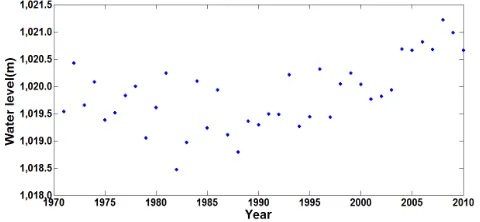
Figure 2. Hystorical maximum recorded water levels 694
695 Fig. 2. Hystorical maximum recorded water levels.
part, from Nanchangtan to Zaoyuan, does not usually freeze because the bed slope is steep and the water velocity is large, and it only freezes in a very cold winter. The rest of the reach, from Zaoyuan to Mahuanggou, flows from south to north and it often freezes because the slope is gentle and the water velocity is low. The Inner Mongolia reach is located on the north of the Yellow River basin between 106◦100E– 112◦500E, 37◦350N–41◦500N. The total length of the main stream is 830 km, and the total height difference is 162.5 m. The reach is wide with a gentle slope and meandering twists and turns. Although it is located in the middle and lower reaches, the slope of the reach that is under study is close to that at the Yellow River estuary.
3.2 Past ice floods
According to historical data for the Yellow River, ice disas-ters appeared frequently in the past and every year between 1855 and 1949, when dams were destroyed by ice floods 27 times. In the period between 1951 and 1955, the dams on the Lijing breach were also destroyed by ice flood. In addition, there were 28 ice flood seasons with ice disasters between 1951 and 2005 (Rao et al., 2012).
Especially on the Ning–Meng reach, ice jams, frazil jams, and other ice flood disasters have happened frequently. Ac-cording to the statistics for ice flood disasters on the Ning– Meng reach, there were 13 ice flood events from 1901 to 1949, almost one event every 4 years. Even after the Liujiaxia Reservoir and the Qingtongxia Reservoir started operation in 1968 and 1960 respectively, ice flood disasters still occurred in 1993, 1996, 2003, and 2008 (Gao et al., 2012).
[image:4.595.51.286.64.244.2]the maximum recorded water levels, every decade between 1970 and 2009, at Sanhuhekou hydrological station.
The Yellow River basin is under the influence of cold air from the vicinity of Siberia and Mongolia; the mean air tem-perature during the whole winter is below 0◦, and this lasts for 4 to 5 months. Due to the special geographical location and difference in latitude of the Ning–Meng reach on the Yel-low River, together with the special river fYel-low direction, the downstream part both freezes and breaks up earlier than the upstream part. Hence it is very easy for ice jams or backwa-ter to be formed, which can result in ice flood disasbackwa-ters such as dams being destroyed and dike breaks. Based on the liter-ature review on ice flood disasters, one can conclude that on the Yellow River the main problems regarding ice floods are caused by ice-dam floods and ice-jam floods which can result in dike breaks and overtopping on the embankment. This is the key problem to be solved on the Ning–Meng reach of the Yellow River.
4 Modelling application
4.1 Model set-up
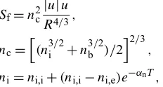
Present research uses the YRIDM, which is a 1-D unsteady-state model. The YRIDM is based on the RICE and RICEN models, and designed taking river ice processes into account. The YRIDM model is simulating the ice dynamics, by de-scribing the skim ice formation and frazil ice as it is in the RICE model. Skim ice formation is based on the empirical equation, developed by Matousek (1984); frazil ice along the river channel is described by the mathematical model defined by Shen and Chiang (1984) and the ice dynamics is described by the static border of the ice formation, which is defined by Svensson et al. (1989) in form of a critical value. The other elements of the ice dynamics are the growth of the border ice, the undercover accumulation, erosion of the ice, and ero-sion of the ice cover due to thermal growth. Though YRIDM is based on the RICE model, there is a major difference in how the break-up of the ice is checked in the two models. In the case of RICE, the critical value of discharge for which the break-up appears is a constant value that has to be deter-mined before using the model, by experiments on site, while in the YRIDM model the critical discharge is determined by an empirical equation.
The YRIDM model was designed to simulate the ice flood for unsteady-state flow, which uses the governing Eqs. (1)– (5) below:
∂A ∂t +
∂Q
∂x =0, (1)
∂Q ∂t +
∂ Q2/A
∂x = −gA ∂Z
∂x +Sf
, (2)
Sf=n2c |u|u
R4/3, (3)
nc=
h
(n3/2i +n3/2b )/2i2/3, (4) ni=ni,i+(ni,i−ni,e)e−αnT, (5)
whereQ= discharge (m3s−1);A= net flow cross-sectional area (m2); x= distance (m); t= time (s); g= gravitational acceleration (m s−2); Sf= friction slope; nc= equivalent
roughness; ni= roughness of ice cover; nb= roughness of
river bed; u= average velocity (m s−1); R= river hydraulic
radius (m); ni,i= initial roughness of ice cover; ni,e= final
roughness of ice cover at the end of an ice-covered period (0.008∼0.012); T= freeze-up time (day); and αn= decay
coefficient.
The YRIDM equations for ice transportation model are different from the ones in RICE, that is, YRIDM uses convection–diffusion equation between ice run and floating ice, while RICE uses a two-layer mode for the surface ice transportation. The critical value of discharge for which the break-up appears is determined by the empirical Eq. (6): Q≥9.5∗a∗hi
P Ta++1
, (6)
whereQis discharge (m3s−1);hiis the ice cover thickness
when air temperature varies from positive values to negative ones (m); a is the break-up coefficient (a=4 for mechanical break-up anda=22 for thermal break-up); andTa+is the
av-erage daily accumulated positive air temperature, measured from the day when air temperature turns positive.
The roughness of ice cover is usually computed based on the end roughness of ice cover and a decay constant; how-ever, the YRIDM model is developed with a constant initial roughness of ice cover, which has been determined by YRCC through several measuring campaigns.
[image:5.595.308.424.58.120.2]The logical flowchart of the YRIDM model is presented in Fig. 3. It consists of three main components, the river hydro-dynamics, thermohydro-dynamics, and ice dynamic modules. The advantage of this model is that it can be subdivided even fur-ther into the following modules: river hydraulics, heat ex-change, water temperature and ice concentration distribu-tions, ice cover formation, ice transport and cover progres-sion, undercover deposition and eroprogres-sion, and thermal growth and decay of ice covers.
1230 C. Fu et al.: Challenges in modelling river flow and ice regime
31 696
697 698
Figure 3. YRCC River Ice Dynamic Model Flowchart 699
700 701 702
703
Figure 4. Verification of the model: Water levels 704
Fig. 3. YRCC river ice dynamic model flowchart.
31 696
697 698
Figure 3. YRCC River Ice Dynamic Model Flowchart
699
700 701 702
703
Figure 4. Verification of the model: Water levels
704
Fig. 4. Verification of the model: water levels.
model, and the winter from 2007 to 2008 was used to verify the calibrated model.
The reach between Bayangaole station and Toudaoguai station was chosen to be modelled due to the fact that ice flood has happened frequently here and data was available on the reach. The simulation reach has a total length of 475.6 km. A hydrological station named Sanhuhekou is po-sitioned in the middle of the reach (i.e. 205.6 km away from Bayangaole station).
The available data includes river hydraulics, meteorologi-cal, ice regime, and cross sectional data at the four hydromet-ric stations, namely Shizuishan, Bayangaole, Sanhuhekou, Toudaoguai stations, and it covers the period of ten win-ters, from 2001 to 2011. River hydraulic data includes wa-ter level and discharge with daily measuring frequency. Me-teorological data includes air and water temperature with a daily measurement of the water temperature and twice a day measurement of air temperature (the daily highest and lowest temperature per day). Ice regime data includes ice run data, freeze-up date, break-up date, and ice cover thickness. The measured frequency is per winter except that the measured
32 705
706 707
708
Figure 5. Verification of the model: Discharge
709
710 711 712
713
Figure 6. Verification of the model: Water temperature
714
715
Fig. 5. Verification of the model: discharge.
32
705 706 707
708
Figure 5. Verification of the model: Discharge 709
710 711 712
713
Figure 6. Verification of the model: Water temperature 714
715
Fig. 6. Verification of the model: water temperature.
frequency of ice cover thickness is every 5 days. Data for four cross sections for 2009 is available.
During the winter of 2008/2009 the discharge and wa-ter temperature at Bayangaole station, the wawa-ter level at Toudaoguai station, air temperature at Sanhuhekou and Toudaoguai stations, and cross sections and bed elevation were used to build the model.
4.2 Model calibration and verification
Table 1. Results of the sensitivity analysis of the parameters of the YRCC river ice dynamic model.
Sensitivity
parameters Physical meaning Reference range Unit Sensitive object
Nb Bed roughness 0.019∼0.045 – Water level
ni,e End-ice roughness 0.008∼0.035 – Water level
αn Decay constant 0.005∼0.4 1/day Water level
Coe_Cw Heat exchange coefficient between water and ice 15∼18 – –
Coe_Hia Heat exchange coefficient between ice and air 6∼12 – Ice cover thickness Coe_Co Heat exchange coefficient between water and air 15∼25 – Ice cover thickness
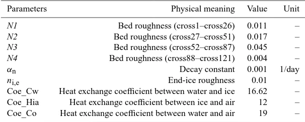
Table 2. Calibrated parameters values.
Parameters Physical meaning Value Unit
N1 Bed roughness (cross1–cross26) 0.011 –
N2 Bed roughness (cross27–cross51) 0.017 –
N3 Bed roughness (cross52–cross87) 0.045 –
N4 Bed roughness (cross88–cross121) 0.004 –
αn Decay constant 0.001 1/day
ni,e End-ice roughness 0.01 –
Coe_Cw Heat exchange coefficient between water and ice 16.62 – Coe_Hia Heat exchange coefficient between ice and air 12 – Coe_Co Heat exchange coefficient between water and air 19 –
Based on the literature review and the reference book of the numerical model from YRCC, the sensitivity parameters are listed in Table 1. The one-at-a-time sensitivity measure method was used to conduct the sensitivity analysis, which means the value of one parameter is changed from the min-imum value to the maxmin-imum value while at the same time other parameters are kept constant at the mean value, and then the variation of the model output is checked.
After the sensitivity analysis, scenarios of the model cal-ibration can be designed based on the sensitivity analysis results (Table 1). If the model is sensitive to a certain pa-rameter, then the parameter needs to be calibrated carefully, otherwise the default value is used. In this case, bed rough-ness, end-ice roughrough-ness, and decay constant are sensitive to the water level at the Sanhuhekou station; heat exchange co-efficient between ice and air, and heat exchange coco-efficient between water and air are sensitive to ice cover thickness at the Sanhuhekou station. These five parameters should be cal-ibrated carefully; the heat exchange coefficient between wa-ter and ice is not sensitive to the output, hence the default value can be set. The model can be calibrated under differ-ent ice regime conditions, which means that some parame-ters can be calibrated under open water conditions, such as the Manning coefficient of river beds and the heat exchange coefficient between water and air. Some parameters can be calibrated under ice conditions, such as the Manning coef-ficient under ice cover, end-ice roughness, and decay con-stant. Hence the model calibration procedure is divided into a model calibration under open water conditions and a model
calibration under ice conditions. In the calibration procedure, RMSE (root mean square error) is used as the criterion to check the model performance.
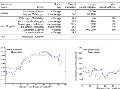
The calibrated bed roughness for different cross sections was varied for a large range of values (i.e from 0.004 to 0.017). These values are provided by YRCC and reflects the four different types of channel beds of the modelled river reach. The Ningxia River reach, which is 397 km long, starts at Nanchangtan and ends at Mahuanggou, in Shizuishan city. From Nanchangtan to Zaoyuan (ca. 135 km) there is an un-common freezing state of the river reach, because the bed slope is steep and water velocity is high. This state allows the river reach to freeze up only during very cold winters. On the reach from Zaoyuan to Mahuanggou (ca. 262 km), on the other hand, there is a common freezing state of the river reach because the slope is gentle and water velocity is small. The Inner Mongolia reach is located on the north of Yellow River basin and has a total length of 830 km. The reach is wide with gentle slopes, meandering twists and turns. Although it is located in the middle and lower Yellow River, its slope is close to that of the Yellow River estuary. A summary of the slopes, width and roughness of these four types of considered reaches is given in the Table 3.
[image:7.595.145.448.219.341.2]1232 C. Fu et al.: Challenges in modelling river flow and ice regime
Table 3. Channel characteristics of Ning–Meng reach.
Autonomous Channel Channel Average Main Channel
region Section type length (km) channel width (m) channel width (m) slope (‰) Roughness
Ningxia Nanchangtan–Zaoyuan valley type 135 200–300 0.8–1.0 0.005–0.014
Zaoyuan–Mahuanggou transition type 262 500–1000 0.1–0.2 0.005–0.014
Inner Mongolia
Mahuanggou–Wuda bridge valley type 69.0 400 400 0.56 0.011–0.020
Wuda bridge–Sanshenggong transition type 106.6 1800 600 0.15 0.011–0.020
Sanshenggong–Sanhuhekou wandering type 205.6 3500 750 0.17 0.009–0.018
Sanhuhekou–Zhaojunfen transition type 126.2 4000 710 0.12 0.009–0.018
Zhaojunfen–Lamawan bend type 214.1 3000–2000 600 0.10 0.002–0.010
Lamawan–Yushuwan valley type 118.5 0.002–0.010
Total Nanchangtan–Yushuwan 1237
33
[image:8.595.260.543.77.373.2]716
Figure 7. Water levels at Sanhuhekou station
717
718
Figure 8. Discharge at Sanhuhekou station
719
Fig. 7. Water levels at Sanhuhekou station.
water level, discharge, water temperature, and ice cover thickness at the Sanhuhekou station during the winter of 2007/2008 were used to compare with the observed values to verify the calibrated model.
The simulation period used for verification of the model was done for the available data from 1 November 2007 to 31 December 2007. Results of the verification are presented in Figs. 4, 5 and 6 for water level, discharge and temperature, respectively. Though there was just little data measured and available for verification, results shows that the model could capture the trend of water level, discharge, and water tem-perature. It is worth to be noted that in 2008/2009, the water level did not exceed the embankments.
4.3 Model uncertainty analysis
Based on the sensitivity analysis results, the water level at the Sanhuhekou station is sensitive to the Manning coefficient of river bed, decay constant, and end-ice roughness; and the ice cover thickness at the Sanhuhekou station is sensitive to the heat exchange coefficient between ice and air, and heat exchange coefficient between water and air. Hence, the un-certainty analysis is divided into an unun-certainty analysis of the water level at the Sanhuhekou station and the uncertainty analysis of ice cover thickness at the Sanhuhekou station, and
33
716
Figure 7. Water levels at Sanhuhekou station 717
718
Figure 8. Discharge at Sanhuhekou station 719 Fig. 8. Discharge at Sanhuhekou station.
the Monte Carlo simulation is used to conduct the parametric uncertainty analysis (Moya Gomez et al., 2013).
Due to the limitation of time, it was impossible to run the model several times. When conducting the uncertainty anal-ysis of the water level at the Sanhuhekou station, the related four parameters were the Manning coefficients of the river bed at the upstream and downstream of the Sanhuhekou sta-tion, decay constant, and end-ice roughness. The scenarios of the uncertainty analysis of the water level at the Sanhuhekou station were designed based on the calibrated parameters, the range was calculated by increasing and decreasing the cali-brated value by 20 %, the sample generation was uniformly random, and the number of simulation was 500. When con-ducting the uncertainty analysis of the ice cover thickness at the Sanhuhekou station, the two related parameters were the heat exchange coefficient between ice and air, and the heat exchange coefficient between water and air. The scenarios of the uncertainty analysis about ice cover thickness at the Sanhuhekou station were designed based on the calibrated parameters, the range was calculated through increasing and decreasing the calibrated value by 20 %, the sample genera-tion was uniformly random, and the number of simulagenera-tions was 400.
34
Figure 9. Water temperature at Sanhuhekou station 720
721
722
Figure 10. Ice cover thickness at Sanhuhekou station 723
Fig. 9. Water temperature at Sanhuhekou station.
34
Figure 9. Water temperature at Sanhuhekou station
720
721
722
Figure 10. Ice cover thickness at Sanhuhekou station
723 Fig. 10. Ice cover thickness at Sanhuhekou station.
stored, the distribution and quartile of the output were anal-ysed, namely the pdf (probability density function) at one time step and two bounds (5 and 95 %).
5 Results and discussion
The results of the sensitivity analysis show that bed rough-ness, end-ice roughrough-ness, and the decay constant are sensitive to the water level at the Sanhuhekou station, and that the heat exchange coefficient between ice and air, and the heat ex-change coefficient between water and air are sensitive to ice cover thickness at the Sanhuhekou station.
Based on the results of the sensitivity analysis, the model was calibrated, and the values of calibrated parameters can be seen in Table 2.
Figure 7 shows the water level comparison at the San-huhekou station during the winter of 2008/2009 between the simulated data and observed data. The resulting RMSE is 0.464. The simulated result is acceptable and reasonable. From day 1 to day 40 the simulated result is not good, but the trend in the simulated results is consistent with the ob-served results, which is because in the beginning, the simu-lated water level is affected by the initial conditions. From
35
724
Figure 11. Water levels at Sanhuhekou station 725
726
Figure 12. Probability distribution of the water level on Day 90 727
Fig. 11. Water levels at Sanhuhekou station.
35
724
Figure 11. Water levels at Sanhuhekou station 725
726
Figure 12. Probability distribution of the water level on Day 90 727 Fig. 12. Probability distribution of the water level on Day 90.
day 125 to the end, the simulated result is not accurate and the trend is even adverse, which is because the model can-not simulate an ice-jam break-up during the break-up period. The data observed during the period clearly shows that the water level decreases suddenly, which means that the ice jam at the downstream of the Sanhuhekou station collapses, but the model cannot simulate this phenomenon, which is why the simulated results are not so accurate. During the rest of the period, the results are acceptable.
1234 C. Fu et al.: Challenges in modelling river flow and ice regime
36
728
Figure 13.Probability distribution of water level on Day 130 729
730
Figure 14. Ice cover thickness at Sanhuhekou station 731
732
Fig. 13. Probability distribution of water level on Day 130.
36
728
Figure 13.Probability distribution of water level on Day 130 729
730
Figure 14. Ice cover thickness at Sanhuhekou station 731
732
Fig. 14. Ice cover thickness at Sanhuhekou station.
model ignores the effect on the water body mass balance due to changes in the ice phase; this is the reason why the results are not good enough. During the other period, the result is acceptable.
Figure 9 shows the comparison between the simulated data and observed data for the water temperature at the San-huhekou station during the winter of 2008/2009; the RMSE is 0.854. The simulated results are acceptable and reasonable. From day 1 to day 15, the simulated results are not good, which is because in the beginning, the simulated water tem-perature is affected by the initial water temtem-perature. From day 55 to day 95, the water temperature is below 0◦; this is the super cooling phenomenon, which means before the for-mation of ice cover the water body loses heat very quickly, which can result in the negative value for the water tempera-ture. However, once the ice cover forms, it can prevent heat exchange between the water body and the air; this is the rea-son why the water temperature keeps steady at 0◦between day 100 and day 130. During the rest of the period, the re-sults are acceptable.
Figure 10 shows the comparison between the simulated data and observed data for ice cover thickness at the San-huhekou station during the winter of 2008/2009. Because the ice cover thickness data was measured per five days, the observed ice cover thickness data is not continuous and
37 733
734
Figure 15. Probability distribution of ice cover thickness on Day 60
735
736
737
Figure 16. Probability distribution of ice cover thickness on Day 120
738
739 740 741
Fig. 15. Probability distribution of ice cover thickness on Day 60.
37 733
734
Figure 15. Probability distribution of ice cover thickness on Day 60
735
736
737
Figure 16. Probability distribution of ice cover thickness on Day 120
738
739 740 741
Fig. 16. Probability distribution of ice cover thickness on Day 120.
the RMSE between the simulated data and observed data is 0.109 m. The simulated results can describe the variation trend for ice cover thickness, and the simulated maximum value of the ice cover thickness, 0.58 m on 28 January 2009, has the same value as the measured one
The prepared data during the winter of 2007/2008 were input into the model to verify the calibrated model. In the winter of 2007/2008, the water level exceeded the height of embankment at Duguitalakuisu county, and resulted in a dike breach, which could not be captured by the model because as per the reference guide for the model, it cannot work when the water level exceeds the height of the embankment. In this respect YRIDM should be improved so that it has the ability to deal with such kind of problems.
least it shows the basic shape of normal distribution, and hence the uncertainty analysis results are reasonable.
After running the model, the uncertainty analysis results can be summarized in Fig. 14. Figure 10 shows the observed data, 5 % percentile bound, 95 % percentile bound, and the results of 400 cases. Day 60 (Fig. 15) and Day 120 (Fig. 16) are chosen to show the probability distribution. According to Figs. 15 and 16, the uncertainty analysis results are not good, due to the fact that the probability distribution of the ice cover thickness on these two days is not a normal distribution. This result is due to the fact that the number of cases designed for the uncertainty analysis might not be sufficient to show the characteristics of a model uncertainty.
Results show the sensitivity of bed roughness, end-ice roughness, and decay constant to water level at the San-huhekou station; and that both the heat exchange coefficient between ice and air and the heat exchange coefficient be-tween water and air are sensitive to ice cover thickness at the same station. The model however cannot work when the water level exceeds the height of embankments, never-theless reasonable results about uncertainty analysis can be achieved. Based on the obtained results it can be concluded that the model can be applied to the Ning–Meng reach to simulate its ice regime, and once calibrated, it can be used to forecast the ice regime to support decision making, such as on artificial ice-breaking and reservoir regulation
6 Conclusions
Tracking ice formation from observations and combining with numerical model predictions for advanced warning re-quires proper understanding of all scientific issues that play a role. In the case of the Yellow River, ice floods impose a threat every year, which is why the Yellow River Com-mission is putting considerable effort in verifying theoreti-cal formulations with actual field measurements in order to better understand the scientific mechanisms that play a role. Transforming this knowledge into an early warning system that can help save lives is a scientific issue that requires at-tention (Almoradie et al., 2014; Jonoski et al., 2014; Popescu et al., 2012).
Based on the obtained results with the YRIDM model it can be concluded that it is applicable to the Ning–Meng reach for simulating ice regimes, and once calibrated, it can be used to forecast the ice regime to support decision making, such as on artificial ice-breaking and reservoir regulation. There is however a limitation of the YRIDM model that it cannot sim-ulate a mechanical break-up during the break-up period be-cause the effect of ice phase change on the water body mass balance is ignored.
The used model has the advantage that for 10–15 days forecasts of the meteorological data that are used as hydro-logical and hydraulic input into the model, the ice regime can be predicted and support decision making.
As the data collection continues the base to determine the possible times of ice formation and consequently flooding is enlarged and improved (Debolskaya, 2009). Based on ice-formation predictions decision makers can take appropriate measures to reduce the risk of flooding. Flooding during cold season is very important, therefore determination of the mo-ments of ice formation that could possibly eliminate flood-ing, due to the decisions taken is also an important task in modelling. For ice formation and based on data availability a 1-D model is sufficient to be used; however, for the deter-mination of the flood extent and time of flood occurrence, a more complex model, such as a 1D-2D, needs to be made available (Gichamo et al., 2013; Shen et al., 2008).
Though the present research focussed on ice formation rather than floods it can be generally concluded that the mea-sured elements and frequency should be increased, and as recommendation if floods need to be captured and simulated then the one-dimensional models should be extended to two-dimensional models.
Acknowledgements. The authors acknowledge the support of the Hydrology Bureau of the Yellow River Conservancy Commission for the data used for the present research as well as for the YRIDM The work presented here was partially supported by the Ministry of Water Resources, China through grant no. 201301062-03.
Edited by: A. Gelfan
References
Almoradie, A., Jonoski, A., Stoica, F., Solomatine, D., and Popescu, I.: Web-based flood information system: case study of Somesul-Mare, Romania, J. Environ. Eng. Manage., 12, 1065–1070, 2013. Beltaos, S.: Challenges and opportunities in the study of river ice processes, Proceedings of 19th International Association of Hydraulic Research Symposium on ice, Vancouver, British Columbia, Canada, 1, 29–47, 2008.
Beltaos, S. and Wong, J.: Downstream transition of river ice jams, J. Hydraul. Eng., ASCE, 112, 91–110, 1986.
Blackburn, J. and Hicks, F.: Suitability of dynamic modeling for flood forecasting during ice jam release surge events, J. Cold Reg. Eng., 17, 18–36, 2003.
Calkins, D. J.: Accelerated Ice Growth in Rivers. CRREL Report 79–14, Hanover, NH, US Army, pp. 4, 1979.
Chen, D. L., Liu, J. F., and Zhang, L. N.: Application of Statistical Forecast Models on Ice Conditions in the Ningxia-Inner Mongo-lia Reach of the Yellow River, Proceedings of 21th International Association of Hydraulic Research Symposium on ice, Dalian, China, 443–454, 2012.
1236 C. Fu et al.: Challenges in modelling river flow and ice regime
Daly, S. F.: Frazil ice dynamics. CRREL Monograph 84-1, US Army CRREL, Hanover, N. H., 1984.
Dahlke, H. E., Lyon, S. W., Stedinger, J. R., Rosqvist, G., and Jans-son, P.: Contrasting trends in floods for two sub-arctic catch-ments in northern Sweden – does glacier presence matter?, Hy-drol. Earth Syst. Sci., 16, 2123–2141, doi:10.5194/hess-16-2123-2012, 2012.
Debolskaya, E. I.: “Numerical Modeling of Ice Regime in Rivers”, Hydrologic Systems Modeling, Vol. 1, Encyclopedia of Life Sup-port Systems, Eolss Publishers, Oxford (UK), 137–165, 2009. Gao, G. M., Yu, G. Q., Wang, Z. L., and Li, S. X.: Advances in
Break-up Date Forecasting Model Research in the Ningxia-Inner Mongolia Reach of the Yellow River, Proceedings of 21th Inter-national Association of Hydraulic Research Symposium on ice, Dalian, China, 475–482, 2012.
Gichamo, T., Jonoski, A., Popescu, I., Morris, M., and Hassan, M.: Embankment failure modeling using HR Breach Model, J. Envi-ron. Eng. Manage., 12, 865–874, 2013.
Hammar, L., Shen, H. T., Evers, K.-U., Kolerski, T., Yuan, Y., and Sobaczak, L: A laboratory study on freeze up ice runs in river channels. Ice in the Environments: Proceedings of 16th Interna-tional Association of Hydraulic Research Symposium on ice, 3, Dunedin, 36–39, 2002
Haresign, M. and Clark, S.: Modeling Ice Formation on the Red River near Netley Cut. CGU HS Committee on River Ice Pro-cesses and the Environment, 16th Workshop on River Ice, Win-nipeg, Manitoba, 147–160, 2011
Jasek, M.: Ice jam release surges, ice runs, and breaking fronts: field measurements, physical descriptions, and research needs, Can. J. Civil Eng., 30, 113–127, 2003.
Jonoski, A., Almoradie, A., Khan, K., Popescu, I., and Andel, S. J.: Google Android Mobile Phone Applications for Water Qual-ity Information Management, J. Hydroinform., 15, 1137–1149, 2013.
Kivisild, H. R.: Hydrodynamic analysis of ice floods, Proceedings of 8th International Association of Hydraulic Research Congress, Montreal, 1959.
Lal, A. M. W. and Shen, H. T.: A Mathematical Model for River Ice Processes, J. Hydraul. Eng., ASCE, 177, 851–867, also USA Cold Regions Research and Engineering Laboratory, CRREL Report 93-4, 1993.
Li, H., Jasek, M., and Shen, H. T.: Numerical Simulation Of Peace River Ice Conditions, Proceedings of 16th International Associ-ation of Hydraulic Research Symposium on ice, Dunedin, New Zealand, Vol. 1, 134–141, 2002
Liu, C. J., Yu, H., and Ma, X. M.:Ice flood in Northeast region. 15th International Symposium on Ice, Gdansk, Poland, 303–312, 2000.
Liu, L. and Shen, H. T.: A two-Dimensional Comprehensive River Ice Model. Proceedings of 18th International Association of Hy-draulic Research Symposium on ice, Sapporo, Japan, 69–76, 2006.
Liu, L. W. and Shen, H. T.: Dynamics of ice jam release surges, Proceedings of 17th International Association of Hydraulic Re-search Symposium on ice, Saint Petersburg, Russia, pp. 8, 2004. Mahabir, C., Hicks, F. E., and Robinson Fayek, A.: Forecasting Ice Jam Risk At Fort Mcmurray, AB, Using Fuzzy Logic, Proceed-ings of 16th International Association of Hydraulic Research Symposium on ice, Dunedin, New Zealand, Vol. 1, 91–98, 2002.
Mahabir, C. F., Hicks, F. E., and Robinson Fayek, A.: Neuro-fuzzy river ice breakup forecasting system, J. Cold Reg. Sci. Technol., 46, 100–112, 2006.
Malenchak, J., Doering, J., Shen, H. T., and Morris, M.,: Numerical Simulation of Ice Conditions on the Nelson River, Proceedings of 19th International Association of Hydraulic Research Sympo-sium on ice, Vancouver, British Columbia, Canada, Vol. 1, 251– 262, 2008.
Moya-Gomez, V., Popescu, I., Solomatine, D., and Bociort, L.: Cloud and cluster computing in uncertainty analysis of integrated flood models, J. Hydroinform., 15, 55–69, 2013.
Morris, M., Malenchak, J., and Groeneveld, J.: Thermodynamic Modeling to Test the potential for Anchor Ice Growth in post-construction conditions on the Nelson River, Proceedings of 19th International Association of Hydraulic Research Sympo-sium on ice, Vancouver, British Columbia, Canada, Vol. 1, 263– 272, 2008.
Osterkemp, T. E.: Frazil ice formation : A review, J.Hydraul. Div., ASCE, 104, 1239–1255, 1978.
Petrow, Th., Merz, B., Lindenschmidt, K.-E., and Thieken, A. H.: Aspects of seasonality and flood generating circulation pat-terns in a mountainous catchment in south-eastern Germany, Hy-drol. Earth Syst. Sci., 11, 1455–1468, doi:10.5194/hess-11-1455-2007, 2007.
Popescu, I., Jonoski, A., and Bociort, L.: Decision Support Systems for flood management in the Timis-Bega catchement, J. Environ. Eng. Manage., 11, 847–953, 2012.
Rao, S. Q., Yang, T. Q., Liu, J. F., and Chen, D. L.: Characteristics of Ice Regime in the Upper Yellow River in the last Ten Years, Proceedings of 21th International Association of Hydraulic Re-search Symposium on ice, Dalian, China, 390–396, 2012. Rojas, R., Feyen, L., Dosio, A., and Bavera, D.: Improving
pan-European hydrological simulation of extreme events through sta-tistical bias correction of RCM-driven climate simulations, Hy-drol. Earth Syst. Sci., 15, 2599–2620, doi:10.5194/hess-15-2599-2011, 2011.
She, Y. and Hicks, F.: Modeling ice jam release waves with consid-eration for ice effects, J. Cold Reg. Sci. Technol., 45, 137–147, 2006.
Shen, H. T. and Chiang, L. A.: Simulation of growth and decay of river ice cover, J. Hydraul. Div., Am. Soc. Civ. Eng., 110, 958– 971, 1984.
Shen, H. T. and Lal, A. M. W.: Growth and decay of river ice covers. Proc., Cold Regions Hydrology Symp., AWRA, Fairbanks, 583– 591, 1986.
Shen, H. T., Su, J., and Liu, L.: SPH Simulation of River Ice Dy-namics, J. Comput. Phys., 165, 752–771, 2006.
Shen, H. T.: A trip through the life of river ice – research progress and needs, Keynote lecture, Proceedings of 18th International Association of Hydraulic Research Symposium on ice, Sapporo, Japan, 2006.
Shen, H. T., Gao, L., Kolerski, T., and Liu, L.: Dynamics of Ice Jam Formation and Release, J. Coast. Res., SI 52, 25–32, 2008. Shen, H. T.: Mathematical modeling of river ice processes, Cold
Reg. Sci. Technol., 62, 3–13, 2010.
Shen, H. T. and Wang, D. S.: Under cover transport and accumu-lation of frazil granules, J. Hydraul. Eng., ASCE, 120, 184–194, 1995.
Shen, H. T., Wang, D. S., and Lal, A. M. W.: Numerical simula-tion of river ice processes, J. Cold Reg. Eng., ASCE 9, 107–118, 1995.
Shen, H. T. and Yapa, P. D.: A unified degree-day method for river ice cover thickness simulation, Can. J. Civil Eng., 12, 54–62, 1985.
Stefan, J.: Uber die theorien des eisbildung insbesondere uber die eisbildung in polarmure, Wien Sitzungsberichte Akademie der Wissenschaften, Series A, 42, 965–983, 1889.
Tesaker, E: Accumulation of frazil ice in an intake reservoir, Proc., IAHR Symposium on Ice problems, Hanover, NH, 1975. Tuthill, A. M., Wuebben, J. L., and Gagnon, J. G.: ICETHK
Users Manual, Version 1, Special Report 98-11, US Army Cold Regions Research and Engineering Laboratory, Hanover, New Hampshire, 1998.
USACE: HEC-2 Water Surface Profiles, Hydrologic Engineering Center, US Army Corps of Engineers, Davis, California, 1992. USACE: HEC-RAS River Analysis System: Hydraulic Reference
Manual, Hydrologic Engineering Center, US Army Corps of En-gineers, Davis, California, June, 1998.
Wang, T., Yang, K., and Guo, Y.: Application of Artificial Neural Networks to forecasting ice conditions of the Yellow River in the Inner Mongolia Reach, J. Hydrol. Eng., ASCE, 13, 811–816, 2008.