Optimisation of LiDAR derived terrain models for river flow modelling

www.hydrol-earth-syst-sci.net/13/1453/2009/ © Author(s) 2009. This work is distributed under the Creative Commons Attribution 3.0 License.

Earth System

Sciences

Optimisation of LiDAR derived terrain models for river flow

modelling

G. Mandlburger1, C. Hauer2, B. H¨ofle3, H. Habersack2, and N. Pfeifer3

1_{Christian Doppler Laboratory “Spatial Data from Laser Scanning and Remote Sensing” at the Institute of Photogrammetry} and Remote Sensing, Vienna University of Technology, Gusshausstrasse 27–29, 1040 Vienna, Austria

2_{Institute of Water Management, Hydrology and Hydraulic Engineering, BOKU – University of Applied Life Sciences,} Muthgasse 107, 1190 Vienna, Austria

3_{Institute of Photogrammetry and Remote Sensing, Vienna University of Technology, Gusshausstrasse 27–29,} 1040 Vienna, Austria

Received: 7 October 2008 – Published in Hydrol. Earth Syst. Sci. Discuss.: 16 December 2008 Revised: 23 June 2009 – Accepted: 3 August 2009 – Published: 14 August 2009

Abstract. Airborne LiDAR (Light Detection And Rang-ing) combines cost efficiency, high degree of automation, high point density of typically 1–10 points per m2and height accuracy of better than ±15 cm. For all these reasons Li-DAR is particularly suitable for deriving precise Digital Ter-rain Models (DTM) as geometric basis for hydrodynamic-numerical (HN) simulations. The application of LiDAR for river flow modelling requires a series of preprocessing steps. Terrain points have to be filtered and merged with river bed data, e.g. from echo sounding. Then, a smooth Digital Ter-rain Model of the Watercourse (DTM-W) needs to be de-rived, preferably considering the random measurement er-ror during surface interpolation. In a subsequent step, a hy-draulic computation mesh has to be constructed. Hyhy-draulic simulation software is often restricted to a limited number of nodes and elements, thus, data reduction and data condition-ing of the high resolution LiDAR DTM-W becomes neces-sary. We will present a DTM thinning approach based on adaptive TIN refinement which allows a very effective com-pression of the point data (more than 95% in flood plains and up to 90% in steep areas) while preserving the most relevant topographic features (height tolerance±20 cm). Traditional hydraulic mesh generators focus primarily on physical as-pects of the computation grid like aspect ratio, expansion ra-tio and angle criterion. They often neglect the detailed shape of the topography as provided by LiDAR data. In contrast, our approach considers both the high geometric resolution of

Correspondence to: G. Mandlburger

([email protected])

the LiDAR data and additional mesh quality parameters. It will be shown that the modelling results (flood extents, flow velocities, etc.) can vary remarkably by the availability of surface details. Thus, the inclusion of such geometric details in the hydraulic computation meshes is gaining importance in river flow modelling.

1 Introduction

Hydrodynamic-numerical (HN) modelling – also referred to as Computational Fluid Dynamic (CFD) modelling – is widespread in water sciences. Simulation tools are used for ecological studies (Hauer et al., 2008a,b) as well as for hy-draulic engineering purposes such as river restoration and the like (Denoth, 2003; Gouda et al., 2002; Khan and Barkdoll, 2000; Fischer-Antze et al., 2001). Moreover, the precise de-lineation of endangered or vulnerable areas in flood hazard analysis is also based on hydrodynamic-numerical models (Habersack and Gaul, 2008). In many countries, land use regulations and building codes are directly linked to flood hazard maps, which show areas affected by events with a cer-tain return period.

flood levels (HQ10/20/50/100/200/500) following uniform technical guidelines (Hoydal et al., 2002). In Austria haz-ard zone maps are developed at a scale of 1 : 2000, in which three zones (red, yellow and blue) are distinguished (RIWA-T, 2006). Red zones are determined by a velocity-depth cri-terion, whereas yellow zones are bounded by the extent of a hundred-years flood. Blue zones exhibit areas of specific flood management. Additionally, rest risk areas (HQ300) and the spatial extent of the thirty year event (HQ30) are pre-sented in Austrian flood hazard mapping (RIWA-T, 2006). Given the importance of event simulations for planning, their quality is crucial.

The most influential input parameters for HN models are the topography provided as a Digital Terrain Model of the Watercourse (DTM-W) and the flow resistances usually pro-vided as roughness coefficients. According to technical advances in computer aided hydrodynamic-numerical mod-elling and the related multidimensional (2-D/3-D) applica-tions, the need for high quality 3-D terrain data is increasing (Sinha et al., 1998). Airborne LiDAR (Light Detection and Ranging) provides high point density and remarkable height precision (Csanyi and Toth, 2007). It is especially well suited for capturing flood plains as well as river banks under low flow conditions and is therefore widely used as data basis for HN models.

However, the application of LiDAR poses problems as well. Contrary to traditional manual data acquisition tech-niques like stereo-photogrammetry or tachymetry, LiDAR data includes both terrain and off-terrain points on buildings, vegetation, power lines, etc. The quality of the derived DTM and, consequently, the quality of subsequent HN modelling depends crucially on how well off-terrain points have been eliminated within the filtering process. Another issue besides filtering is the fusion of LiDAR and river bed data. This volves the derivation of the water-land-boundary and the in-terpolation of river bed cross sections.

Nowadays, most HN models are solved using a Finite Ele-ment (FE) or Finite Volume (FV) approach on the basis of un-structured or hybrid geometries, i.e. a computation grid based on irregularly distributed points. Many hydraulic mesh gen-erators are available, which build up a net of polygonal sur-face elements covering the entire project area. Mainly trian-gles and arbitrary quadrilaterals are in use. Hereby, the ver-tices of the quadrilaterals don’t need to be co-planar. These mesh generators consider hydraulic parameters like angle criterion and aspect ratio, but normally disregard topographic details as contained in data from modern LiDAR sensors. The heights are mapped to the hydraulic grid a posteriori. Many modelling tools can only handle a limited number of points and elements (Nujic, 1999). Thus, the direct use of the high resolution LiDAR DTM as computation grid is impos-sible due to the enormous amount of data.

This article presents a new method for constructing hy-draulic computation grids by preserving geometric surface details as well as considering physical mesh quality

param-0 100 200 300 400 500 600 700 800 900

04.08.2002 00:00

06.08.2002 00:00

08.08.2002 00:00

10.08.2002 00:00

12.08.2002 00:00

14.08.2002 00:00

16.08.2002 00:00

18.08.2002 00:00

discharge (m

3/s)

Q1 max = 800 m 3

/s

Q2 max = 488 m 3

/s catstrophic flood 2002 one-year event

HQ100

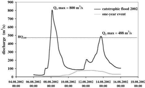
Fig. 1. Hydrograph recorded at gauging station Stiefern during the

catatstrophic flood in August 2002 (6–16 August) featuring two peaks (800 m3/s on Aug 8; 488 m3/s on 15 August) (black line); hydrograph of a one-year flood at gauging station Stiefern (grey line); the hydrographs are compared to the discharge of a 100-year flood (Q=470 m3/s, black dashed line).

eters. An adaptive TIN refinement method is used to thin out the high resolution LiDAR DTM, which is professionally conditioned in a subsequent postprocessing step to meet the required mesh quality parameters. The method, thus, over-comes the limitations of mesh generation approaches con-sidering physical parameters only.

In the following Sect. 2 the study area and data sets are introduced. Thereafter, the major steps of the proposed workflow are described in detail, comprising LiDAR DTM processing (Sect. 3), DTM data reduction and conditioning (Sect. 4) and hydrodynamic-numerical modelling (Sect. 5). The results and application examples are presented and dis-cussed in the subsequent Sects. 6 and 7. The final section concludes the major findings and points out the benefits of our approach.

2 Study area and data sets

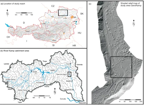
Fig. 2. (a) Map of Austria including the river Kamp system; (b) catchment area of the river Kamp with main tributaries (E 15◦260, N 48◦320; extension: 47 km×23 km); (c) River section (Gars am Kamp), shaded relief map of the Digital Surface Model.

in the Kamp valley chute cut-offs and floodplain stripping occurred and local overbank scours were documented.

The study reach is a 2 km section midstream of the river Kamp situated in the northern part of Lower Austria at the village Gars am Kamp (Fig. 2). The origin of the river Kamp is near the village Karlstift and after a 160 km long course it discharges into the Danube River (182 m a.m.s.l.) at Al-tenw¨orth. The total catchment area measures 1753 km2and the hydrologic regime is described as pluvio-nival (Mader et al., 1996) with an average annual precipitation of 900 mm. The average bed slope of the selected study reach is ap-prox. 2.5‰. The investigated river section of Gars am Kamp was heavily affected by the catastrophic flooding in August 2002. A high percentage of buildings (20.1%, 293 of 1460) were damaged or even destroyed. As entire losses a sum of more than 13 million C was reported by the Lower Austrian Federal Government (Habersack et al., 2004).

As a result of the extreme 2002 flood event a LiDAR campaign was carried out for the entire Kamp valley. The

3 LiDAR DTM processing

In this section the state of the art in DTM acquisition in gen-eral and obtaining terrain models from airborne LiDAR in particular will be reviewed.

For the specification of terrain surface products the Dig-ital Terrain Elevation Data (DTED) levels from 1 to 5 have been suggested. For HN simulations especially the resolu-tion and accuracy levels are of interest. Level 2 is fulfilled by DTMs with a horizontal resolution (grid edge length) of 100 (approx. 20–30 m) and an absolute vertical accuracy of 18 m (90% error bound). It may be reached by spaceborne Interferometric Synthetic Aperture Radar (InSAR) using the X-band (e.g. SRTM, Rabus et al., 2003), which is, however, scattered back at the tree crowns. Level 3, also referred to as High Resolution Terrain Information (HRTI-3), with 12 m resolution and 10 m accuracy, is aimed at by new satellite InSAR missions (Krieger et al., 2007). HRTI-4 (6 m resolu-tion, 5 m accuracy) can be achieved by airborne InSAR and stereo photogrammetry (Kraus, 2007). At this level it makes a notable difference if the ground surface is recorded or the first visible surface from the bird’s perspective (tree crowns, roofs, etc.). Short wavelength radar and passive optical imag-ing can provide high resolution, but cannot take measure-ments from the ground surface below the forest cover (Balt-savias et al., 2008). HRTI-5 can currently only be provided by airborne LiDAR for larger areas in a cost efficient manner and prescribes a resolution of 1 m, an absolute vertical accu-racy of 5 m, and a relative (point-to-point) precision of 25 cm. Especially the accuracy requirements are the fact advocating for airborne LiDAR.

In airborne LiDAR the travel time of a short pulse of laser energy from the sensor to the ground surface and back is measured. The position and orientation of the sensor plat-form is determined with GNSS and IMU (Global Navigation Satellite System, Inertial Measurement Unit). The laser pulse can “see” through small gaps in the foliage and travel to the ground below the tree canopy. The result is a cloud of points originating from the ground surface and the canopy in a for-est environment. In open areas the points are only lying on the ground surface. The task of separating the points on the ground surface from the other, off-terrain points is called fil-tering (Kraus and Pfeifer, 1998). Different approaches have been suggested (Pfeifer and Mandlburger, 2008) making dif-ferent assumptions on the terrain surface and either proceed by gradually adding or by gradually removing unclassified points. Finally, advanced algorithms also consider the ran-dom measurement noise.

The methods of mathematical morphology (Kilian et al., 1996; Vosselman, 2000; Zhang et al., 2003) classify points depending on vertical and horizontal distances between points. The principle is that a large height difference at small horizontal distance can only occur, if the higher point is off the ground. In progressive densification (von Hansen and V¨ogtle, 1999; Axelsson, 2000; Sohn and Dowman, 2002) the

terrain surface is described by a triangulation, that is gradu-ally built up. Starting from a few known terrain points, new points are added, if they are within certain distances from the triangulation surface. With these algorithms also a notion of surface is introduced. In robust interpolation (Kraus and Pfeifer, 1998) a surface model is interpolated starting from all points, more precisely approximating all points, e.g. by linear prediction or kriging (Kraus, 2000; Journel and Hui-jbregts, 1978). This surface model runs in an averaging way between terrain and off-terrain points. The residuals, i.e. the vertical distances from the measurements to the surface model, are computed and become input for a weight func-tion. This way, high weights are associated with points be-low the current surface, and small weights with points above it. These weights are considered in the next iteration step of surface computation. Points with larger weights attract the surface, while points with lower weights have less and less influence in subsequent iterations. The approach has been embedded in a hierarchic setup, for increasing robustness and efficiency (Pfeifer et al., 2001). A comparable method has been suggested by Elmqvist et al. (2001). The advantage of this approach is that the surface properties, expressed e.g. by the variogram of kriging, are clearly separated from the prop-erties of LiDAR data (terrain and off-terrain points), which are expressed in the weight function. Random measurement errors are considered, if a suitable surface interpolation tech-nique like linear prediction is chosen. Finally, segmentation approaches were suggested (Sithole and Vosselman, 2005; Nardinocchi et al., 2003; T´ovari and Pfeifer, 2005) for sep-arating terrain and off-terrain points, which first group the points to larger entities (e.g. planar areas) and then classify those. They are mainly advantageous in city areas, where a large number of well-defined, planar surfaces do exist.

4 DTM data reduction and conditioning

4.1 DTM data reduction

Modern LiDAR sensors allow mapping of topographic de-tails at the price of a highly increased data volume. In order to obtain a manageable amount of data for FE meshes used in HN modelling data reduction and surface simplification is inevitable. The main goal is to reduce the vertices of the DTM (grid points, breaklines, etc.) without losing relevant geometric details.

For polygonal simplification of 2.5-D surfaces mainly reg-ular grid algorithms, decimation and refinement techniques are in use (Heckbert and Garland, 1997). The regular grid approaches are widespread, simple and fast, but they are not adaptive and produce poor approximation results. Better ap-proximation quality can be achieved by applying decimation and refinement methods based on general triangulation algo-rithms such as Delaunay triangulation. Decimation methods work from fine-to-coarse and are not suited for processing large high resolution LiDAR DTMs since they require a tri-angulation of the entire point set. Refinement methods repre-sent a coarse-to-fine approach starting with a minimal initial approximation. In each subsequent pass one or more points are added as vertices to the triangulation until the desired approximation tolerance is met or the desired number of ver-tices is used.

The performance of DTM data reduction is highly influ-enced by the existence of systematic and random measure-ment errors. For deriving thinned DTMs from original Li-DAR point clouds, refinement or decimation approaches as described above are not the first choice. Systematic errors have to be removed first by rigorous sensor calibration and fine adjustment of the LiDAR strip data (Schenk, 2001; Filin, 2003; Kager, 2004). The random measurement errors of the LiDAR points should rather be eliminated by applying a DTM interpolation strategy with measurement noise filter-ing capabilities such as linear prediction (Kraus, 2000) or kriging (Journel and Huijbregts, 1978). High reduction ra-tios can only be achieved for DTMs, where systematic errors have been strictly eliminated and random errors have been reduced during surface interpolation.

In contrast to approaches which rely on the original point cloud, our adaptive TIN refinement approach uses the filtered hybrid DTM (regular grid and breaklines, structure lines, and spot heights) as input (Mandlburger, 2006). The basic pa-rameters for the DTM simplification are a maximum height error1zmax(L∞-norm) and a maximum planimetric point

distance1xymax. The latter avoids triangles with too long edges and narrow angles. The algorithm starts with an ini-tial approximation of the DTM comprising all structure lines and a coarse regular grid (cellsize=1xymax=10), which are triangulated using a Constrained Delaunay Triangulation. Each 10-cell is subsequently refined by iteratively

insert-ing additional grid points until the height tolerance1zmax is reached.

The additional vertices can either be inserted hierarchi-cally or irregularly. In case of a hierarchical breakdown, a coarse rectangular grid is used as initial surface approxima-tion. Each coarse grid cell is divided into four parts in each pass, if a single grid point within the regarded area exceeds the maximum tolerance. This leads to a quad-tree like point distribution in the resulting surface approximation. By con-trast, for irregular division a regular grid of (approximately) equilateral triangles is used as initial approximation. This is especially suited for FE-meshes since the connecting line of adjacent cell centers (i.e. direction of calculation) always in-tersects the joint cell boundary at a right angle. In a single pass the grid points with the maximum positive and maxi-mum negative deviation are inserted (parallel greedy inser-tion). Furthermore, the process of point insertion and recal-culation of the error measures is optimised by considering the locality of the mesh changes. Higher compression ratios (up to 99% in flat areas) can be achieved with irregular point insertion, whereas the hierarchical mode is characterised by a more homogeneous vertex distribution. The hierarchic di-vision, thus, produces an adaptive cartesian grid whereas ir-regular division yields an unstructured grid.

4.2 Data conditioning

To get a high quality computation grid for HN modelling, the simplified polygonal surface mesh has to be conditioned considering the physical phenomena being simulated (flow direction, bottom shear stress, . . . ). According to Ferziger and Peric (2002) the main quality parameters for a good FE grid are: (i) angle criterion, (ii) aspect ratio and (iii) expan-sion ratio. The aspect ratio describes the proportion of the longest and shortest edge within a mesh face, whereas the ex-pansion ratio is a measure describing the area ratio between adjacent faces. Requirements concerning angles in a compu-tational mesh appear in two different ways. First, the angles between the mesh edges and, second, the alignment of the cells with respect to the direction of force have to be consid-ered. Ferziger and Peric (2002) report that small angles of less than 10◦should be avoided, the cells should be aligned to the principal flow direction, the aspect ratio should not ex-ceed 10 (optimum<3) and the expansion ratio must not be greater than 3 (optimum<1.2).

embankment, the flow directions are no longer strictly paral-lel, thus, irregular data distribution as described in the previ-ous subsection is appropriate.

However, especially for flood mapping different zones can be designated within the inundation area depending on the respective vulnerability. Residential areas in the vicinity of a river, for instance, should be mapped in more detail than re-mote or elevated areas. The concept of varying mapping pre-cisions can be applied to the DTM simplification approach by introducing spatially varying maximum height tolerances. Mathematically the tolerances can be expressed as a bivariate function (1zmax=f (x, y)). Distances from the river bank or relative height differences, respectively, can be used to con-trol the tolerances, but a simple zonal model has turned out to be suited best. The delineation of the different accuracy zones can be derived from a pilot survey (e.g. a preliminary 1-D-CFD simulation), from DTM visualisations such as hill shadings, from existing maps or the like.

Finally, the resulting TIN has to be analysed with respect to the adherence of angle criterion, aspect and expansion ra-tio. Therefore, the entire triangulation is traversed and, if necessary, additional vertices are inserted or hydraulically unessential vertices are removed. Figure 3 shows the original high resolution LiDAR DTM-W whereas a simplified grid, professionally conditioned to preserve geometric details and fulfill physical quality criterions, is illustrated in Fig. 4.

5 Hydrodynamic-numerical modelling

To evaluate the impact concerning the availability of geo-metric details on the results of river flow simulations, the two-dimensional depth-averaged hydrodynamic-numerical model Hydro AS-2-D (Nujic, 1999) was applied in the study reach. Basic principles of two-dimensional mathematical flow modelling are the 2-D depth-averaged equations (sim-plified Navier-Stokes-equations), also referred to as shallow-water equations. Within the Hydro AS-2-D model the shal-low water equations are spatially discretised based on the fi-nite volume approach. Simplified in vector form the shallow water equation can be described as follows:

∂w

∂t +

∂f

∂x +

∂g

∂y +s=0 (1)

where:

w=





H uh vh



, f = 

 

uh

u2h+gh2

2 −νh ∂u ∂x

uvh−νh_∂x∂v



 ,

s=





0

gh(IRx−ISx)

gh(IRy−ISy)



, g= 

 

vh

uvh−νh∂u_∂y

v2h+gh2

2 −νh ∂v ∂y



 

His the water surface elevation [m], the sum of the water depth (h) and the terrain height (z).uandvare the velocities in x- and y-direction [m/s],gthe acceleration due to gravity [m/s2] andνthe kinematic viscosity term [m2/s].

IRx =

λu

√

u2_+v2

2gD , IRy = λv

√

u2_+v2

2gD

ISx = −

∂z

∂x, ISy = −

∂z ∂y

λ=6.342gn

2

3

√

D

where,nis the Manning coefficient [√3s_m],Dthe hydraulic

diameter 4Rhy[m],Rhy=H=water depth [m].

Hydro AS-2-D uses the Surface water Modelling System (SMS) as a pre- and postprocessing tool. The convective flow of the two-dimensional model is based on the Upwind-scheme by Pironneau (1989) and the discretisation of time is done by an explicit Runge Kutta method in second or-der. Several methods for implementing viscosity in numeri-cal modelling exist. In the applied Hydro AS-2-D model the viscosity is calculated based on a combination of empirical and constant viscosity approaches.

ν=ν0cµv∗h (2)

wherecµis the viscosity parameter andv∗the shear velocity [m/s] andν0is a basic viscosity term.

In the applied Hydro AS-2D modelν0 is used to ensure numerical stability. In general, different ν0-values can be assigned to each cell, but in practice ν0 is only adapted in sections. For the simulations in this case study no ν0 adaption was employed at all, a viscosity coefficient of

Fig. 3. Perspecitve view of the final 1 m DTM-W of Gars am Kamp including the Dungl hotel (image center), buildings are considered as

block models and integrated as breaklines into the hybrid grid.

Fig. 4. Perspective view of a professionally thinned and conditioned DTM-W grid, which also serves as hybrid hydraulic computation mesh

be considered in the summarizing roughnessn-value. Any-way, due to the lack of reference data it is not the aim of the presented paper to achieve validated flood stages for the hundred-years event by calibrating different overbank pa-rameters (e.g. vegetation, land use, . . . ) but rather to show the impact of geometry details provided by LiDAR on the modelling results.

6 Results

Before running the hydrodynamic-numerical simulation we had to build up a precise LiDAR based DTM-W covering the wetted perimeter of a HQ100 at least and including the river bed and all flow prohibiting buildings. Our data basis comprised the LiDAR points aligned in a 1 m raster, the river bed cross sections (terrestrial survey) and 2-D building poly-gons (cadastral map). In a first step, we derived a DTM of the overbank areas without gaps. Since the LiDAR terrain points at hand were sparsely distributed due to prior filtering, we merged all terrain and DSM points and analysed the point cloud with SCOP++ (SCOP++, 2009), which implements the hierarchic robust interpolation (c.f. Sect. 3). Thereafter, we derived the water-land-boundary as described in Brockmann and Mandlburger (2001) serving as clipping polygon to cut out all laser echoes within the river bed. The bed surface itself was subsequently constructed by densifying the cross sections using an interpolation approach, which considers the curved progression of the river axis (Mandlburger, 2000). To reflect the natural flow conditions in our geometry model as realistically as possible, we decided to include the build-ings as block models in the DTM-W. Therefore, we used 2-D building polygons from the cadastral map and estimated an average height for each building. The resulting 3-D polygons were introduced to the DTM-W in a final step, where we interpolated all preprocessed data (i.e. classified LiDAR ter-rain points and densified river bed points) using linear predic-tion (Kraus, 2000). Thus, random measurement errors in the height component in the order of±15 cm were considered in the DTM computation. A grid with an edge length of 1 m containing additional breaklines was derived and the result-ing hybrid DTM-W is illustrated in Fig. 3. Virtually all the tasks mentioned above were carried out using the SCOP++ software developed at the Institute of Photogrammetry and Remote Sensing, Vienna.

Additionally, data reduction and conditioning was per-formed as described in Sect. 4. We chose a maximum height tolerance 1zmax=±20 cm and started the TIN refinement process with a basic triangular point pattern (edge length

10=16 m). The irregular TIN of the river bed was automati-cally replaced by cell elements aligned to the flow direction. The resulting professionally thinned and conditioned DTM-W grid, which can be used as hydraulic computation mesh straightforwardly, is shown in Fig. 4.

1 : 5 0 0

(a)

(b)

Fig. 5. Computation grid of two geometry variants I and II for

G. Mandlburger et al.: Optimisation of LiDAR DTMs for river flow modelling 1461 1 : 5 0 0

(a)

1 : 5 0 0

(b)

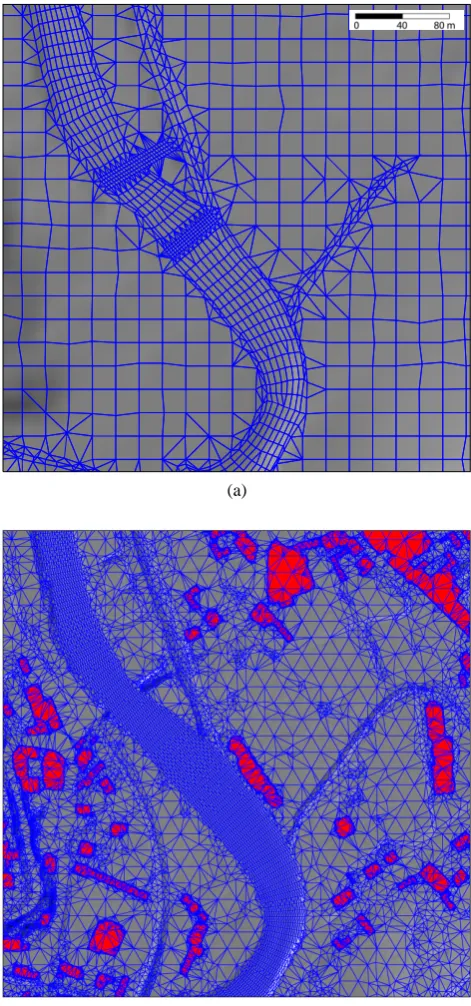
Fig. 5:Computation grid of two geometry variants I and II for HN modelling, Gars/Kamp, Lower Austria;(a)Geometry I: regular20×20 m2

grid, additional breaklines for description of river bank and weir channel, river bed: structured grid;(b)Geometry II: hybrid grid derived

from 1mLiDAR DTM-W via adaptive TIN refinement and subsequent mesh conditioning, river bed and river bank: structured grid (post

spacing 5min flow direction and 2mperpendicular to it), over bank area: unstructured grid: maximum height tolerance∆zmax=±20 cm,

buildings in red.

1 : 5 0 0

(a)

1 : 5 0 0

ra ilw

a y d_a

m

m road

da

(b) [m]

Fig. 6:Flood extents (red boundary line) and water depths [m] for a simulated HQ100 (470m3/s) in Gars/Kamp;(a)extended flooding of

residential area beyond the dams in model I;(b)inundation area restricted by dams (e.g. railway dam) in model II.

Both parameters show a similar progression in both geome-try variants with greater values in model II than in model I. The maximum bottom shear stress values are 129N/m2_{in I} and 211N/m2_{in II which represents a relative increase of}

+63%of model II compared to I.

Finally, the cross section plotted in Fig. 7 was examined in detail and the results concerning water depth, flow velocity and bottom shear stress are illustrated in Fig. 10. The water

Fig. 6. Flood extents (red boundary line) and water depths [m] for a simulated HQ100 (470 m3/s) in Gars/Kamp; (a) extended flooding of

residential area beyond the dams in model I; (b) inundation area restricted by dams (e.g. railway dam) in model II.

10 G. Mandlburger et al.: Optimisation of LiDAR DTMs for river flow modelling

1 : 5 0 0

(a)

1 : 5 0 0

(b) [m/s]

Fig. 7:Flow velocities [m/s] for a simulated HQ100 (470m3/s) in Gars/Kamp;(a)model I shows higher flow velocities in the floodplain

than model II, outline of longitudinal section (red, c.f. Fig. 9) and cross section (yellow, c.f. Fig. 10);(b)main channel: higher velocities in

model II compared to model I, detail window (black, c.f. Fig. 8).

m 10 20

n

o D

u gle _h

te_l

(a)

D un

gl _ho te_l

(b)

0.00 0.12 0.25 0.37 0.50 0.62 0.75 0.87 1.00 1.12 1.25 1.32 1.50 1.62 1.75 1.87 2.00 2.12 2.25 2.37

[m/s]

Fig. 8: Flow vectors of a detailed area around the Dungle hotel for a simulated HQ100 (470m3/s) in Gars/Kamp;(a)model I shows

unrealistic parallel flow vectors within and around the building; (b)flow vectors of model II reflect the secondary currents around the

building correctly.

depth of both model variants exhibit only small deviations in the range of a few centimeters. However, an increase of the flow velocity can be observed in model II within the main channel, which is compensated by lower flow velocities in the over bank areas. Model I shows a reciprocal progression with lower velocities in the main channel and higher values in the foreland. At station 150m, for instance, the velocity adds up to 0.76m/sin model I and only 0.21m/sin II. Fur-thermore, an interesting detail can be observed at the location

computation grid of model II in a generalised way, the wa-ter depth, velocity and bottom shear stress go down to zero. These details are not reflected in the coarser model I.

7 Discussion

Due to the fact, that LiDAR based hydraulic modelling can be seen as state of the art in hazard zone mapping, it should

Fig. 7. Flow velocities [m/s] for a simulated HQ100 (470 m3/s) in Gars/Kamp; (a) model I shows higher flow velocities in the floodplain

than model II, outline of longitudinal section (red, c.f. Fig. 9) and cross section (yellow, c.f. Fig. 10); (b) main channel: higher velocities in model II compared to model I, detail window (black, c.f. Fig. 8).

To estimate the impact of additional topographic details provided by LiDAR on instream hydraulics, numerical sim-ulations for HQ100 were carried out for two different ge-ometry variants. We compared a low resolution gege-ometry I to a very detailed description of the terrain (geometry II). Geometry I consists of a regular 20 m grid. The spatial res-olution conforms to DTED Level 2, which can be achieved using spaceborne remote sensing techniques like InSAR (e.g. SRTM). Anyway, the deployed 20 m grid was derived from LiDAR via static grid reduction (low pass filtering). In a pre-processing step the coarse grid was augmented by additional breaklines from terrestrial survey to improve the description of the river banks and weir channels. By contrast, geome-try II was derived from the precise 1 m LiDAR DTM-W as a hybrid computation grid (floodplain: unstructured grid, river bed: structured grid) as described above. The two different grid variants are illustrated in Fig. 5.

For the investigated 2 km river reach geometry I featured a total number of 6602 nodes (13 091 triangular or quadri-lateral surface elements) whereas geometry II consists of 96 225 nodes (191 229 surface elements). The 1 m LiDAR DTM-W contains a total number of 1.16 million grid posts and 20 600 breakline points (building terrain intersections and eaves). Thus, for geometry I only 0.5% of the avail-able data source are utilised to describe the terrain geometry and, therefore, many surface details are lost. For geometry II 8% of the LiDAR DTM-W posts are necessary to describe the terrain surface with a maximum approximation tolerance

1zmax=±20 cm.

The most important results of hydraulic simulations are water depths, flow velocities and flow direction vectors. Based on these parameters water surface levels, flood extents and bottom shear stresses are derived. Figure 6 contains a map of water depths and flood boundaries for the same sec-tion and the same geometry variants as shown in Fig. 5. A remarkable difference of the flood extent between model I and II can be observed, especially close to the railway dam and the road dams. These geometric details are contained in model II only. They restrict the inundated area whereas the flooded area exceeds beyond the dams in model I. The consequences of the restricted run-off area in model II are illustrated in Fig. 7. It can be seen that the flow velocities in the main channel are higher in model II than in model I compensated by higher overbank flow velocities in model I compared to model II.

Additionally, overbank areas are often characterised by non-parallel water flow. 2-D-HN modelling is the method of first choice for deriving distinct flow directions in each cell element. Figure 8 shows the flow vectors for a detailed area around the Dungl hotel (black window in Fig. 7b). It can clearly be seen that secondary currents around the hotel are well represented in model II whereas unrealistic paral-lel flow vectors even crossing the building can be observed in model I. Moreover, Fig. 8 reveals the above mentioned differences in overbank velocities more clearly. Model I

fea-tures flow velocities within a range of 0.5-0.8 m/s, whereas model II shows values between 0-0.2 m/s.

A more thorough quantitative comparison of the veloc-ity differences of both model variants was carried out for a 215 m long section along the center line of the river Kamp close to the Dungl hotel. The profile outline is plotted in Fig. 7, whereas the velocity profile itself is illustrated in Fig. 9. The mean velocity in model I is 2.17 m/s (sample size n=45) and 3.17 m/s (n=97) in model II. The differ-ence of the mean velocities between model I and II is sta-tistically significant with respect to a 95% confidence inter-val (p=0.0). Figure 9 illustrates the progression of the flow velocity and bottom shear stress (i.e. parameter for erosion and deposition of sediments) along the longitudinal section. Both parameters show a similar progression in both geome-try variants with greater values in model II than in model I. The maximum bottom shear stress values are 129 N/m2in I and 211 N/m2 in II which represents a relative increase of +63% of model II compared to I.

Finally, the cross section plotted in Fig. 7 was examined in detail and the results concerning water depth, flow velocity and bottom shear stress are illustrated in Fig. 10. The water depth of both model variants exhibit only small deviations in the range of a few centimeters. However, an increase of the flow velocity can be observed in model II within the main channel, which is compensated by lower flow velocities in the over bank areas. Model I shows a reciprocal progression with lower velocities in the main channel and higher values in the foreland. At station 150 m, for instance, the velocity adds up to 0.76 m/s in model I and only 0.21 m/s in II. Fur-thermore, an interesting detail can be observed at the location of the Dungl hotel. Since the buildings are contained in the computation grid of model II in a generalised way, the wa-ter depth, velocity and bottom shear stress go down to zero. These details are not reflected in the coarser model I.

7 Discussion

G. Mandlburger et al.: Optimisation of LiDAR DTMs for river flow modelling 1463 1 : 5 0 0

(a)

1 : 5 0 0

(b) [m/s]

Fig. 7:Flow velocities [m/s] for a simulated HQ100 (470m3_/s

) in Gars/Kamp;(a)model I shows higher flow velocities in the floodplain

than model II, outline of longitudinal section (red, c.f. Fig. 9) and cross section (yellow, c.f. Fig. 10);(b)main channel: higher velocities in

model II compared to model I, detail window (black, c.f. Fig. 8).

m 10 20

n

o D

u gle _h

te_l

(a)

D un

gl _ho te_l (b) 0.00 0.12 0.25 0.37 0.50 0.62 0.75 0.87 1.00 1.12 1.25 1.32 1.50 1.62 1.75 1.87 2.00 2.12 2.25 2.37 [m/s]

Fig. 8: Flow vectors of a detailed area around the Dungle hotel for a simulated HQ100 (470m3/s) in Gars/Kamp;(a)model I shows

unrealistic parallel flow vectors within and around the building; (b)flow vectors of model II reflect the secondary currents around the

building correctly.

depth of both model variants exhibit only small deviations in the range of a few centimeters. However, an increase of the flow velocity can be observed in model II within the main channel, which is compensated by lower flow velocities in the over bank areas. Model I shows a reciprocal progression with lower velocities in the main channel and higher values in the foreland. At station 150m, for instance, the velocity adds up to 0.76m/sin model I and only 0.21m/sin II. Fur-thermore, an interesting detail can be observed at the location of the Dungl hotel. Since the buildings are contained in the

computation grid of model II in a generalised way, the wa-ter depth, velocity and bottom shear stress go down to zero. These details are not reflected in the coarser model I.

7 Discussion

Due to the fact, that LiDAR based hydraulic modelling can be seen as state of the art in hazard zone mapping, it should be highlighted that precise and reliable modelling results (i.e. flood extents . . . ) can only be achieved by exploiting the full

Fig. 8. Flow vectors of a detailed area around the Dungle hotel for a simulated HQ100 (470 m3/s) in Gars/Kamp; (a) model I shows

unrealistic parallel flow vectors within and around the building; (b) flow vectors of model II reflect the secondary currents around the building correctly. 150 200 250 3,5 4 4,5 b ot tom s h ear s tr es s [N /m 2] w at er d ep th [ m ], f low ve loc it y [ m /s ] v (I) 0 50 100 2 2,5 3

0 50 100 150 200 250

b ot tom s h ear s tr es s [N /m w at er d ep th [ m ], f low ve loc it y [ m /s ]

downstream distance [m]

v (I) v (II) shear (I) shear (II)

Fig. 9. Flow velocity [m/s] and bottom shear stress [N/m2]

of a longitudinal section for a simulated HQ100 (470 m3/s) in Gars/Kamp. 60 70 80 90 100 6 7 8 9 10 b ot tom s h ear s tr es s [N /m 2] w at er d ep th [ m ], f low ve loc it y [ m /s ] depth (I) depth (II) v (I) Dungl hotel 0 10 20 30 40 50 0 1 2 3 4 5

0 100 200 300 400

b ot tom s h ear s tr es s [N /m w at er d ep th [ m ], f low ve loc it y [ m /s ] station [m] v (I) v (II) shear (I) shear (II)

Fig. 10. Water depth [m], flow velocity [m/s] and bottom shear

stress [N/m2] of a cross section including the Dungl hotel following the left river bank for a simulated HQ100 (470 m3/s) in Gars/Kamp.

The potential discharge area in the village Gars is re-stricted by the railway dam (right bank) and road dams (left bank). For the 100-year flood event the dams act as a flow barrier in model II since they are reflected sufficiently in the computation grid whereas the coarser geometry approxima-tion of model I allows overtopping of the dams and, there-fore, inundating of large flood plain areas beyond the dams. Proper consideration of the dams requires a certain ground resolution of the topographic data acquisition. A resolu-tion of 20–30 m, that can be achieved using spaceborne In-SAR techniques is, therefore, not sufficient for precise hazard zone mapping. Airborne LiDAR, in contrast, is well suited both concerning the required planimetric resolution of ap-prox. 1 m and height accuracy better than 20 cm. The rele-vant flow restricting features can be considered in the com-putation grid either by means of a higher point density at the base and top of the dams or by including the dam break-lines as constraints in the mesh. It has to be mentioned, that in case of the reported 2002 flood the entire area of Gars including the flood plains beyond the dams were inundated, but the discharge of this extreme event was by far higher than the HQ100 discharge for which the simulations at hand were carried out. Furthermore, it should be stressed that the dams were treated as watertight in the simulations, i.e. no culverts were considered. However, openings in dams are nowadays more and more safeguarded by mobile flood control mea-sures.

existing buildings. Many cases of dam breaks and under-mining of building foundations were reported in the recent past (Habersack and Krapesch, 2006).

The findings of the study clearly reveal that hydraulic char-acteristics (e.g. flow vectors) are less realistic in geometry I compared to the LiDAR derived geometry II. The cross-sectional comparisons of flow velocity and bottom shear stress have shown a decrease of these parameters in the pre-cise model variant II compared to the coarse model I for over-bank areas. Maximum bottom shear stress values of up to 10 N/m2can be observed in model I, whereas the values are five times lower (approx. 1–2 N/m2) in II. Low bottom shear stress entails a sedimentation of transported suspended loads. Siltation processes, in turn, can be observed at virtually ev-ery flood event and provoke a high vulnerability particularly for residential areas. Therefore, a correct estimation of flow velocities and bottom shear stresses in hydraulic models can be regarded as equally important as a precise estimation of the flood extent. This becomes even more relevant when us-ing flood hydraulics as boundaries for suspended- and bed load transport modelling. The comparison of the simulation results at hand has shown the high impact of the detailed Li-DAR based geometry description II especially on flow ve-locity and bottom shear stress. It can be stated that a correct representation of these hydraulic modelling parameters can only be achieved on the basis of a precise and detailed de-scription of the geometry.

8 Conclusions

In this article a method for the generation of a hydraulic grid was presented. It starts from a digital terrain model in the form of a regular or hybrid grid, which is derived from air-borne LiDAR point clouds by a method considering the ran-dom measurement errors. An irregular thinning scheme al-lows deriving an irregular triangular mesh considering a user-defined height tolerance compared to the original DTM. In the example presented, the point set describing the terrain was reduced to less than 8% in comparison to the original point cloud and the regular DTM grid. The obtained trian-gular mesh is conditioned by inserting vertices in order to assure that the hydrodynamic numerical simulations can be solved.

Airborne LiDAR allows identifying vegetated areas and buildings. The properties of LiDAR even enable retrieving terrain point measurements below the forest cover and, thus, enable obtaining accurate terrain models. Especially for low vegetation areas, full waveform laser scanning is a step for-ward to increase the reliability of the ground point classifica-tion. The identified building blocks, in turn, can be inserted into the grid for flood event simulation.

A flood event simulation on a grid according to the pro-posed method was compared to a simulation on a regular hy-draulic grid featuring a resolution in the order of 20 m.

Eleva-tion data with similar resoluEleva-tions are available publicly (e.g. SRTM). New spaceborne satellite missions aim at resolutions of a few meter, but the accuracy of airborne LiDAR will not be reached. Additionally, as short wavelengths (X-band) are used, no terrain below forest canopy can be derived.

The two event simulations were similar with respect to their water surface levels but showed remarkable differences concerning the flooded area, flow velocity, etc. Comparisons to real floodings (e.g. suspended sediment deposition, side erosion processes) indicate, that the simulation on the basis of the low resolution elevation information is not realistic.

We conclude therefore that (i) airborne LiDAR is the method of first choice for topographic data acquisition of floodplains, and (ii) that the method of first reducing ran-dom measurement errors and subsequently applying irregular thinning in overbank areas and cell arrangement with respect to the flow direction in the river bed leads to meshes, that need little conditioning such models are well suited as input for HN analysis. This asserts that the geometric information captured by airborne LiDAR is in its essence available for hydrodynamic-numerical simulations.

Acknowledgements. We would like to thank company EVN/grafotech (EVN, 2009) for providing the LiDAR data of the study reach and the Austrian federal office of metrology and surveying (BEV, 2009) for providing the cadastral map, which was used to derive the building models.

Edited by: M. Tedesco

References

ARGE Kamp: Machbarkeitsstudie Hochwasserschutz, Studie im Auftrag der Nieder¨osterreichischen Landesregierung, technical report, Austria, 2005.

Axelsson, P.: DEM generation from laser scanner data using adap-tive TIN models, in: International Archives of Photogrammetry and Remote Sensing, XXXIII, B4, 111–118, Amsterdam, The Netherlands, 2000.

Baltsavias, E., Gruen, A., Eisenbeiss, H., Zhang, L., and Waser, L. T.: High-quality image matching and automated generation of 3D tree models, Int. J. Remote Sens., 29, 1243–1259, 2008. BEV: Bundesamt f¨ur Eich- und Vermessungswesen, online

avail-able at: http://www.bev.gv.at/, 2009.

Brockmann, H. and Mandlburger, G.: Modelling a watercourse DTM based on airborne laser-scanner data – using the example of the River Oder along the German/Polish Border, in: Proceed-ings of OEEPE Workshop on Airborne Laserscanning and Inter-ferometric SAR for Detailed Digital Terrain Models, Stockholm, Sweden, 2001.

Csanyi, N. and Toth, C.: Improvement of Lidar data accuracy using lidar-specific ground targets, Photogramm. Eng. Remote Sens., 73, 385–396, 2007.

Doneus, M. and Briese, C.: Digital terrain modelling for archaeo-logical interpretation within forested areas using full-waveform laserscanning, in: The 7th International Symposium on Vir-tual Reality, Archaeology and Cultural Heritage VAST, Zypern, 2006.

Elmqvist, M., Jungert, E., Lantz, F., Persson, A., and S¨oderman, U.: Terrain modelling and analysis using laser scanner data, in: International Archives of Photogrammetry and Remote Sensing, XXXIV, 3/W4, Annapolis, MD, USA, 2001.

EVN: Energieversorgung Nieder¨osterreich AG, online available at: http://www.evn.at/, 2009.

Ferziger, J. H. and Peric, M.: Computational Methods for Fluid Dynamics, Springer, Berlin, Germany, 3 Ed., 2002.

Filin, S.: Recovery of systematic biases in laser altimetry data us-ing natural surfaces, Photogramm. Eng. Remote Sens., 69, 1235– 1242, 2003.

Fischer-Antze, T., Stoesser, T., Bates, P., and Olsen, N.: 3D numer-ical modelling of open channel flow with submerged vegetation, J. Hydraul. Res., 39, 303–310, 2001.

Gouda, M., Karner, K., and Tatschl, R.: Dam flooding simulation using advanced CFD methods, in: Proceedings of the Fifth World Congress on Computational Mechanics, Vienna, Austria, 2002. Gutknecht, D., Reszler, C., and Bl¨oschl, G.: The August 7, 2002 –

flood of the Kamp – a first assessment, Elektrotechnik und Infor-mationstechnik, 119, 411–413, 2002.

Habersack, H.: Mathematische Modelle offener Gerinne, Sonder-druck des Konstruktiven Landschafts-Wasserbaus, Band 17, Vi-enna, Austria, 1995.

Habersack, H. and Gaul, A. (eds.): Fließgew¨assermodellierung – Arbeitsbehelf Hydrodynamik, Nr. 37, ¨Osterreichische Wasser-und Abfallwirtschaftsverband, Vienna, Austria, 2008.

Habersack, H. and Krapesch, G.: Hochwasser 2005 – Teilbericht der Bundeswasserbauverwaltung, Bundesministerium f¨ur Land-und Forstwirtschaft, Umwelt Land-und Wasserwirtschaft, Universit¨at f¨ur Bodenkultur, Wien, 2006.

Habersack, H., B¨urgel, J., and Petraschek, A.: Analyse der Hochwasserereignisse vom August 2002, floodrisk, Synthese-bericht, 2004.

Hauer, C., Mandlburger, G., and Habersack, H.: Hydraulically re-lated hydro-morphological units: description based on a new conceptual mesohabitat evaluation model (MEM) using LiDAR data as geometric input, River Res. Appl., 279–296, online avail-able at: http://www3.interscience.wiley.com/journal/117953086/ abstract, 2008a.

Hauer, C., Unfer, G., Schmutz, S., and Habersack, H.: Morphody-namic Effects on the Habitat of Juvenile Cyprinids (Chondros-toma nasus) in a restored Austrian Lowland River, Environ. Man-age., 42, 279–296, 2008b.

Heckbert, P. S. and Garland, M.: Survey of Polygonal Surface Sim-plification Algorithms, Tech. rep., School of Computer Science, Carnegie Mellon University, Pittsburgh, PA, Technical Report, 1997.

Holzmann, H.: Ereignisdokumentation Hochwasser August 2002, aP-Hydrologie, Habersack & Moser, 2002.

Hoydal, O. A., Berg, H., Haddenland, I., Petterson, L. E., Vosko, A., and Oydvin, E.: Procedures and guidelines for flood inundation maps in Norway, Norwegian Water and Energy Directorate, 404– 410, 2002.

Journel, A. G. and Huijbregts, C. J.: Mining Geostatistics,

Aca-demic Press, New York, USA, 1978.

Kager, H.: Discrepancies Between Overlapping Laser Scanning Strips – Simultaneous Fitting of Aerial Laser Scanner Strips, in: International Archives of Photogrammetry and Remote Sensing, XXXV, B/1, Istanbul, Turkey, 555–560,2004.

Khan, A. A. and Barkdoll, B.: Two-Dimensional Depth-Averaged Models for Flow Simulation in River Bends, Int. J. Comput. Eng. Sci., 2, 453–467, 2000.

Kilian, J., Haala, N., and Englich, M.: Capture and evaluation of airborne laser scanner data, in: International Archives of Pho-togrammetry and Remote Sensing, XXXI, B3, Vienna, Austria, 383–388, 1996.

Kraus, K.: Photogrammetrie, Band 3, Topographische Information-ssysteme, D¨ummler, 2000.

Kraus, K.: Photogrammetry – Geometry from Images and Laser Scans, de Gruyter, 2 Ed., 2007.

Kraus, K. and Pfeifer, N.: Determination of Terrain Models in Wooded Areas with Airborne Laser Scanner Data, ISPRS J. Pho-togramm. Remote. Sens., 53, 193–203, 1998.

Krieger, G., Moreira, A., Fiedler, H., Hajnsek, I., Werner, M., You-nis, M., and Zink, M.: TanDEM-X: A Satellite Formation for High-Resolution SAR Interferometry, IEEE T. Geosci. Remote, 45, 3317–3341, 2007.

Mader, H., Steidl, T., and Wimmer, R.: Klimatologisch-Hydrologische Typisierung der ¨Osterreichischen Fließgew¨asser, Umweltbundesamt, Wien, Austria, 1996.

Mandlburger, G.: Verdichtung von Echolot-Querprofilen unter Ber¨ucksichtigung der Flussmorphologie, ¨Osterr. Z. Vermessung & Geoinformation, 4, 211–214, 2000.

Mandlburger, G.: Topographische Modelle f¨ur Anwendungen in Hydraulik und Hydrologie, Ph.D. thesis, Vienna University of Technology, Austria, 2006.

Marco, J. B.: Flood risk mapping, Kluwer Academic Publishers, Dordrecht, The Netherlands, 353–373, 1994.

Menendez, M.: Design discharge calculations and flood plain management, European Comission (Directorate, General XII), Cemagref, 53–82, 2000.

Nardinocchi, C., Forlani, G., and Zingaretti, P.: Classification and Filtering of Laser Data, in: International Archives of Photogram-metry and Remote Sensing, XXXIV, 3/W13, Dresden, Germany, 2003.

Nujic, M.: Praktischer Einsatz eines hochgenauen Verfahrens f¨ur die Berechnung von tiefengemittelten Str¨omungen, Ph.D. thesis, Universit¨at der Bundeswehr M¨unchen, Institut f¨ur Wasserwesen, Prof. W. Bechteler (superv.), Mitteilungen Nr. 62, 1999. Petraschek, A.: Risk assessment and hazard zone planning in

Switzerland, ¨Osterr. Wasser- und Abfallwirtschaft, 54, 123–127, 2002.

Pfeifer, N. and Mandlburger, G.: Topographic Laser Ranging and Scanning: Principles and Processing, chap. Filtering and DTM Generation, CRC Press, 2008.

Pfeifer, N., Stadler, P., and Briese, C.: Derivation of Digital Terrain Models in the SCOP++ Environment, in: Proceedings of OEEPE Workshop on Airborne Laserscanning and Interferometric SAR for Detailed Digital Terrain Models, Stockholm, Sweden, 2001. Pironneau, P.: Finite Element Methods for Fluids, Masson, Paris,

1989.

acquired by spaceborne radar, ISPRS J. Photogramm. Remote Sens., 57, 241–262, 2003.

RIWA-T: Technische Richtlinien f¨ur die Bundeswasserbauverwal-tung, Bundesministerium f¨ur Land- und Forstwirtschaft, Umwelt und Wasserwirtschaft, 2006.

Schenk, T.: Modeling and recovering systematic errors in airborne laser scanners, in: Proceedings of OEEPE Workshop on Air-borne Laserscanning and Interferometric SAR for Detailed Dig-ital Terrain Models, Stockholm, Sweden, 2001.

SCOP++: Institute of Photogrammetry and Remote Sensing, on-line available at: www.ipf.tuwien.ac.at/products/products.html, 2009.

Sinha, S., Sotiropoulus, F., and Odgaard, A.: Three-dimensional nu-merical model for flow through natural rivers, J. Hydraulic Eng., 124, 14–24, 1998.

Sithole, G. and Vosselman, G.: Experimental comparison of filter-ing algorithms for bare-earth extraction from airborne laser scan-ning point clouds, ISPRS J. Photogramm. Remote Sens., 59, 85– 101, 2004.

Sithole, G. and Vosselman, G.: Filtering of airborne laser scanner data based on segmented point clouds, in: International Archives of Photogrammetry and Remote Sensing, XXXVI, 3/W19, En-schede, The Netherlands, 66–71, 2005.

Sohn, G. and Dowman, I.: Terrain surface reconstruction by the use of tetrahedron model with the MDL Criterion, in: In-ternational Archives of Photogrammetry and Remote Sensing, XXXIV, Graz, Austria, 3B, 336–344, 2002.

TopoSys: Topographische Systemdaten GmbH, online available at: http://www.toposys.de/, 2009.

T´ovari, D. and Pfeifer, N.: Segmentation based robust interpola-tion – a new approach to laser data filtering, in: Internainterpola-tional Archives of Photogrammetry and Remote Sensing, XXXVI, En-schede, The Netherlands, 3/W19, 79–84, 2005.

von Hansen, W. and V¨ogtle, T.: Extraktion der Gel¨andeoberfl¨ache aus flugzeuggetragenen Laserscanner-Aufnahmen, Photogram-metrie Fernerkundung Geoinformation, 4, 229–236, 1999. Vosselman, G.: Slope based filtering of laser altimetry data, in:

In-ternational Archives of Photogrammetry and Remote Sensing, Amsterdam, Netherlands, XXXIII, B3, 935–942, 2000. Wagner, W., Ullrich, A., Melzer, T., Briese, C., and Kraus, K.:

From single-pulse to full-waveform airborne laser scanners: po-tential and practical challenges, in: International Archives of Photogrammetry and Remote Sensing, Istanbul, Turkey, XXXV, 2004.

Watt, W.: Twenty Years of Flood Risk Mapping Under Canadian National Damage Reduction Program, Kluwer Academic Pub-lishers, Dordrecht, The Netherlands, 155–165, 2000.