Uncertainty analysis of hydrological ensemble forecasts in a distributed model utilising short range rainfall prediction

(1)

Earth System

Sciences

Uncertainty analysis of hydrological ensemble forecasts in a

distributed model utilising short-range rainfall prediction

Y. Xuan1, I. D. Cluckie2, and Y. Wang3

1_{Dept. of Hydroinformatics and Knowledge Management, UNESCO-IHE Institute for Water Education, 2611 AX,}

Delft, The Netherlands

2_{Water and Environmental Management Research Centre (WEMRC), Dept. of Civil Engineering, University of Bristol,}

Bristol, BS8 1UP, UK

3_{Taiwan Typhoon and Flood Research Institute, Taichung 40763, Taiwan}

Received: 12 June 2006 – Published in Hydrol. Earth Syst. Sci. Discuss.: 19 October 2006 Revised: 8 December 2008 – Accepted: 8 February 2009 – Published: 6 March 2009

Abstract. Advances in mesoscale numerical weather pred-ication make it possible to provide rainfall forecasts along with many other data fields at increasingly higher spatial resolutions. It is currently possible to incorporate high-resolution NWPs directly into flood forecasting systems in order to obtain an extended lead time. It is recognised, how-ever, that direct application of rainfall outputs from the NWP model can contribute considerable uncertainty to the final river flow forecasts as the uncertainties inherent in the NWP are propagated into hydrological domains and can also be magnified by the scaling process. As the ensemble weather forecast has become operationally available, it is of particu-lar interest to the hydrologist to investigate both the poten-tial and implication of ensemble rainfall inputs to the hy-drological modelling systems in terms of uncertainty prop-agation. In this paper, we employ a distributed hydrologi-cal model to analyse the performance of the ensemble flow forecasts based on the ensemble rainfall inputs from a short-range high-resolution mesoscale weather model. The results show that: (1) The hydrological model driven by QPF can produce forecasts comparable with those from a raingauge-driven one; (2) The ensemble hydrological forecast is able to disseminate abundant information with regard to the nature of the weather system and the confidence of the forecast it-self; and (3) the uncertainties as well as systematic biases are sometimes significant and, as such, extra effort needs to be made to improve the quality of such a system.

Correspondence to: Y. Xuan

([email protected])

1 Introduction

With advances in numerical weather prediction (NWP) in re-cent years as well as an increase in computing power, it is now possible to generate very high resolution rainfall casts at the catchment scale and therefore, more flood fore-casting systems are tending to utilise quantitative precipita-tion predicprecipita-tion (QPF) from high-resoluprecipita-tion NWPs in order to extend the forecast lead time. This is particularly true in the flash flooding area where the model performance is highly dependent on the rapid availability of knowledge of rainfall distribution in advance (Ferraris et al., 2002). Many efforts have been made to utilise the QPF in the context of real-time flood forecasting in which one or more “state-of-the-art” QPFs stemming from different methods are to be integrated into the whole system (e.g. Bartholmes and Todini, 2005; de Roo et al., 2003; Kobold and Suˇselj , 2005; Verbunt et al., 2006; Xuan et al., 2005; Xuan and Cluckie, 2006). However, the effects of QPF uncertainty on the whole system can be easily appreciated either intuitively or by case studies (Xuan et al., 2005). Indeed, recent research on integrating QPF di-rectly into the real-time flood forecasting domain reveals that direct coupling of the QPF with the hydrological model can result in large bias and uncertainty which can result in not only severe underestimation (Bartholmes and Todini, 2005; Kobold and Suˇselj , 2005) but over predicting as well, espe-cially for mountainous areas (Verbunt et al., 2006) .

(2)

1.1 The weather model component

The weather models, which are routinely run in national weather centres, have such a coarse spatial resolution that hydrological models have difficulty applying the result from them as an effective input. The so-called downscaling pro-cedure is needed to bridge the scale gap between the large-scale weather forecast domains and catchment-sized flood forecasting domains. In this study, a dynamical-downscaling approach is applied to resolve the dynamics over 2 km grids. The forecasts/analyses from global weather models are used to settle the initial and lateral boundary conditions (IC/LBC) of a mesoscale model that is able to benefit from the resolv-able terrain features and physics at higher resolutions. This sort of mesoscale model is often referred to as a local area model (LAM).

Lorenz (1963, 1993) introduced the concept that the time evolution of a nonlinear, deterministic dynamical system, to which the atmosphere (essentially a boundary layer process) and the equations that describe air motion belong, are very sensitive to the initial conditions of the system. The uncer-tainties inherited in the larger scale model, which provides the parent domain with the IC and LBC, can also be propa-gated to the nested mesoscale models. Given the large num-ber of degrees of freedom of the atmospheric phase state, it is impractical to directly generate solutions of the probabilis-tic equations of initial states (Kalnay, 2002). The ensemble forecast method, runs the model separately over a probabilis-tically generated ensemble of initial states, each of which represents a plausible and equally likely state of the atmo-sphere, and projects them into future phase space. As such the future state-space can be represented by the statistics of the ensemble.

1.2 The hydrological model component

The hydrological model, like weather models, is subject to the same factors regarding the uncertainty sources in weather modelling systems. For a stand-alone hydrological model, although uncertainties in data inputs, e.g., measurements or observations, have been regarded as one of the main sources of uncertainty, the model structure and parameterisations have drawn more attention from hydrologists (Wagener et al., 2001). Simply speaking, the uncertainty related to hydrolog-ical modelling is categorised as: that from the inability to obtain the state of the system and that due to inefficient mod-elling of reality.

As for the coupling system discussed here, it is important to recognise that the rainfall input uncertainty may always outweigh the impact of the model structure, owing to the fact that the inputs are not directly measured; rather, they are the direct outputs and already include a certain amount of un-certainty which can be magnified by a particular coupling process.

1.3 The objective of this study

Considerable research effort has been made on both NWP based QPF and the application of NWP in flood forecasting (e.g. Smith and Austin, 2000). The objective of this paper, however, is to address uncertainties in ensemble hydrolog-ical forecasting driven by high resolution ensemble rainfall forecasts from the NWP, and to understand the implication of the spatial/temporal variability of rainfall forecasts applied in the flood forecasting environment. To achieve this, we em-ploy a simple distributed hydrological model to investigate the distribution effect of rainfall forecasts and a high resolu-tion rainfall ensemble predicresolu-tion system to provide rainfall forecasts at the catchment scale. A densely-gauged catch-ment with sufficient data records was chosen to run the sim-ulations, and this will be discussed in the following sections.

2 The catchment and models setup 2.1 The Brue catchment

The Brue catchment, located in the South West of England, UK, is an ideal experimental site for research on weather radar, quantitative precipitation forecasting and rainfall-run off modelling, as it has been facilitated with a dense rain gauge network as well as coverage by three weather radars. Numerous studies (Bell and Moore, 2000; Moore et al., 2000; Pedder et al., 2000; Cluckie et al., 2000) have been con-ducted regarding the catchment, notably during the period of the Hydrological Radar EXperiment (HYREX) which was a UK Natural Environment Research Council (NERC) Special Topic Program. Figure 1 shows the locations of the Brue catchment and the gauging stations. The River Brue rises in clay uplands in the east of the catchment. The major land use is pasture on clay soil and there are some patches of wood-land in the higher eastern catchment, which forms part of the unique landscape of the Somerset Levels and Moors.

(3)

# *

5

5 5

5

5 5

5

5 5 5

5

5 5

5

5 5

5

5 5

5

5 5

5

5 5

5

5 5

5

5 5

360000 365000 370000 375000

13

00

13

50

00

14

00

Model Grids 5 _{Rain gauge}

#

* _{Flow gauge} Rivers

Elevation metres

288

[image:3.595.108.483.63.322.2]

2

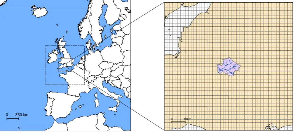
Fig. 1. The Brue catchment and the mesh configured for GBDM model (the horizontal and vertical axes refer to the Easting and Northing in National Grid Reference co-ordinates).

0 350 km

0 10 km

Fig. 2. The domain configuration of the MM5 (left with each domain indicated by dash-dot lines) and the detailed view of domain 4 (right, the Brue catchment shown with colour shade near the centre).

2.2 The hydrological model

A simplified grid-based distributed rainfall-runoff model (GBDM), which is based on the kinematic wave approach,

[image:3.595.49.550.380.609.2]

(4)

and verified using 17 historical storm events over the Brue catchment. The shuffled complex evolution (SCE) method (Duan et al., 1992, 1993, 1994), which is a general-purpose global optimisation strategy designed to solve the various re-sponse surface problems in calibrating a non-linear simula-tion model, was utilised to calibrate the model parameters. 2.3 The short-range ensemble rainfall prediction system A short-range ensemble QPF system was used to produce ensemble rainfall forecasts that can be ingested into the hydrological model to generate the river flow forecasts. The ensemble QPF system was initially implemented in the FLOODRELIEF project and has been used in several case studies (Xuan et al., 2005). The system consists of: the PSU/NCAR mesoscale model (MM5) (Dudhia et al., 2003), the global forecast datasets from the European Centre for Medium-range Weather Forecasts (ECMWF) (Persson, 2003), the model physics selector and a post-processing sys-tem. Using the ensemble approach, the system is capable of representing uncertainties due to perturbations in initial and boundary conditions and the efficiency of the model struc-ture.

In this study, the system was configured to produce en-sembles over a short time range, i.e., 24 h. The model struc-ture was not perturbed in terms of changing physics param-eterisations, as previous research revealed that uncertainties in rainfall forecasts due to parameterisations are not always significant compared with those from inaccuracy of initial and/or boundary conditions (Xuan et al., 2005). The ensem-bles comprise only the direct downscaling of perturbed back-ground fields from ECMWF, i.e., the fifty members of the ECMWF ensemble prediction system, and one operational forecast member which represents the best estimate of the atmospheric state.

In order to reach the spatial scale complementary to the rainfall-runoff modelling system, four nests were used with the inner-most one having a resolution of about 2 km and covering a region around 100 km by 100 km (Fig. 2). The domains were deliberately set so that the target catchment was well centred inside all the nests in order to largely re-duce the effects of spatial distortion owing to different map projections used in weather models and rainfall-runoff mod-els.

3 The simulations

The simulation of this study contains two parts, i.e., the con-ventional calibration and verification of GBDM in respect of the raingauge data; and the simulation with rainfall ensemble inputs to the calibrated hydrological model. We hereby give a brief description of the conventional calibration process and draw more attention to the simulation with ensemble rainfall inputs.

3.1 Calibration of GBDM

The distributed hydrological model used in this study, GBDM, has been calibrated with 13 historical storm events and verified using 4 (see Table 1)that occurred over the Brue catchment from year 1993 to 2000 covering different sea-sons.

The parameters of GBDM can be categorised as two groups, i.e., those physically-based parameters which can be generated directly from topographic, soil, and vegetation maps, and those that need to be calibrated from historical rainfall and flow data. Three calibration parameters (CS, CCandCh, see Appendix) have been calibrated by applying both an optimisation technique and an objective function. In this study, the SCE method was adopted for model calibra-tion. The SCE method is a general-purpose global optimisa-tion strategy designed to solve the various response surface problems encountered in calibrating a non-linear simulation model. Details can be found in Duan et al. (1992, 1993, 1994) .

3.2 The processing of rainfall inputs

Like most hydrological models, the GBDM uses the rain-gauge data for its calibration and verification. Although the model is grid based and has a grid size of 500 m in this case, the rainfall value for each grid was actually obtained using the Thiessen polygon method. When the rainfall forecasts are used to drive the hydrological model, the rainfall val-ues from the weather model were first subject to a projec-tion transformaprojec-tion (from Lambert Conformal projecprojec-tion to National Grid Reference of the UK), and then linear interpo-lation was adopted to transfer the rainfall from 2 km weather model grids to the hydrological grids which have a 500 m grid size.

(5)

6 4 2 0

0 20 40 60 80 100

0 20 40 60

Q (m3/s

)

Rain (mm)

observed Simulated

Time (hours) [Event 14]

3 2 1 0

0 20 40 60 80

0 20 40 60

observed Simulated

Time (hours)

Q (m3/s

)

[image:5.595.54.538.62.408.2] [image:5.595.127.468.484.552.2]

Rain (mm)

[Event 15]

4 3 2 1 0

0 20 40 60 80 100

0 10 20 30 40

Time (hours)

observed Simulated

Q (m3/s

)

Rain (mm)

[Event 16]

observed Simulated 3

2 1 0

0 20 40 60 80 100

0 20 40 60

Time (hours)

Q (m3/s

)

Rain (mm)

[Event 17]

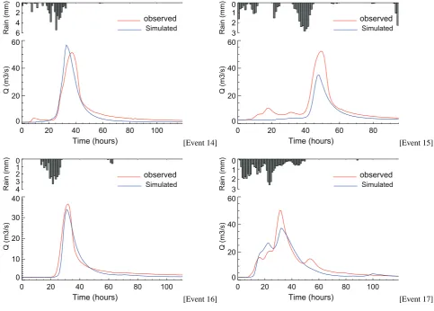
Fig. 3. The verifications of the discharge forecasts for the four events with the observed hourly areal rainfall shown on the top.

Table 1. The verification of GBDM with four history storm events.

Event No. Date Coefficient of model efficiency (CE)

14 23/10/1999 09:00 – 28/10/2000 08:00 0.88

15 17/12/1999 04:00 – 21/12/1999 03:00 0.69

16 31/31/2000 23:00 – 05/02/2000 14:00 0.92

17 02/04/2000 15:00 – 07/04/2000 14:00 0.87

step. For each step, calculate the correlation coefficient of the rainfall forecast extracted by the mask and the reference distribution obtained in the previous step. Therefore, a se-ries of correlation coefficient values are obtained in respect of different offsets ofx andy. After this searching proce-dure, a best matched area has been identified and the data values within this area are available for future processing.

Another common problem relates to the application of the QPF to a hydrological model, where the final forecast can be severely underestimated if applied with a hydrological model calibrated using point rainfall from the raingauges.

(6)

-40 -20 0 20 40 -40

-20 0 20 40

Rmax = 0.36 Rmin = 0.15

-40 -20 0 20 40

[image:6.595.131.464.61.220.2]

Rmax = 0.54 Rmin = 0.40

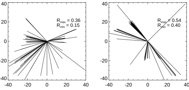
Fig. 4. The shift of mask frame to get the highest correlation coefficient between the rainfall ensemble members and the observed catchment rainfall distribution for events No. 15(a) and No. 16(b) , where the horizontal and vertical axes are shifting in East-West and South-North directions respectively in km. The Origins are the initial locations without shifting.

ratio of the amount obtained in step (1) to the total catchment rainfall value for weather model in the same period. (3) Ad-just the hourly rainfall value from the weather model by the factor obtained in step (2). It should be noted this simple bias correction is a sort of “posterior” method; it is used here for evaluation only and is not suitable for forecasting.

3.3 Test events of ensemble forecasts

The storm events No. 15 and No. 16 were selected for uncer-tainty analysis. Both these events are also the ones for ver-ification of the GBDM with conventional rain gauge inputs. While No. 15 contains several sub-events, No. 16 seems to have one single continuous event which lasts for a longer pe-riod of time.

The original verification results from these events are shown in Fig. 3. It can be seen that the model performed very well for event 16 but under-predicted the main flow peak of event 15. One reason for this is that the GBDM has diffi-culty identifying the transition state of the catchment in the interval in-between two consecutive heavy rainfall inputs.

In order to evaluate the uncertainty of the rainfall forecasts regarding the location, the results of the best match in terms of maximum correlation coefficient are plotted in Fig. 4. Un-der the current configuration, the catchment mask can move within the MM5 innermost domain with a maximum distance inxandydirection of about 80 km. The origins in Fig. 4 are the initial settings, i.e., the original position of catchment. The highest valueRmaxand the lowest oneRminfrom all the

“best-matched” ensemble members are also depicted in the figure for both events.

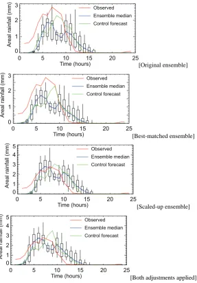
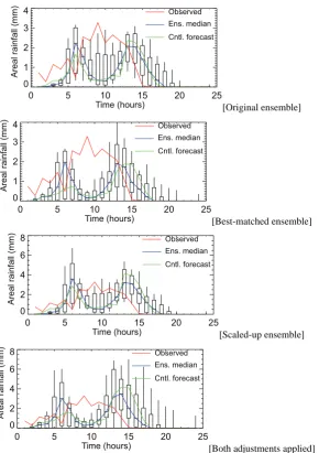
Figures 5 and 6 give the 24 h ensemble rainfall forecasts over the catchment in forms of box plots (Wilks, 1995). Note that in terms of areal rainfall, the median values of the ensem-bles still resemble each other after undergoing the location correction as mentioned above.

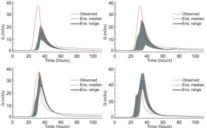
The ensemble rainfall forecasts are then ingested into a time window of 24 h for both events. For event 15, the en-semble rainfall forecast was initialised on 18 December 1999 12:00 UTC and the hourly rainfall forecasts were produced up to 19 December 1999 12:00 UTC, corresponding to the time window from the 34th step to the 57th step. The original rainfall values within this window have then been substituted by the ensemble rainfall forecasts. The same procedure was also applied to event 16 but with a time start of 01 February 2000 12:00 UTC and the corresponding window from step 14 to step 37. The ensemble forecasts are displayed in Fig. 7 and Fig. 8 where the shaded areas represent the spread of all ensemble members between the quantilesq0.1andq0.9. Also

shown are the control forecasts, based on the “best estimate” rainfall forecast results. Note that the rainfall values here are referred to the average of all ensemble members.

4 Discussion

4.1 The direct application of the rainfall ensemble

(7)

Time (hours)

0 5 10 15 20 25

0 1 2 3

Areal rainfall (mm)

Observed

Ensemble median

Control forecast

[Original ensemble]

Time (hours)

0 5 10 15 20 25

0 1 2 3

Areal rainfall (mm)

Observed

Ensemble median

Control forecast

[Best-matched ensemble]

Time (hours)

0 5 10 15 20 25

0 1 2 3 4 5

Areal rainfall (mm)

Observed

Ensemble median

Control forecast

[Scaled-up ensemble]

Areal rainfall (mm)

0 5 10 15 20 25

0 1 2 3 4 5

Time (hours)

Observed

Ensemble median

Control forecast

[image:7.595.155.443.60.473.2]

[Both adjustments applied]

Fig. 5. The box plots of the areal rainfall ensemble forecast of event 15 subject to different adjustments. The lower and upper bounds of the boxes are corresponding to quantilesq0.1andq0.9respectively.

4.2 The dispersion of location and its implications

The introduction of the best match rainfall field pattern in Sect. 3.2 provides a new prospective on the uncertainty of the QPF regarding location. Although this method is defined by the maximum correlation between the rainfall forecast and the reference one, it also reveals the spatial relationship of all ensemble members. We can safely argue that members that agree with each other must have locations close to each other in the “best match” map as in Fig. 4; therefore the dispersion of those locations to some extent can be seen as a indicator of the agreements among ensemble members and as such, im-ply the spread of the trajectories of members in the model’s phase space. However, it is worth noting that due to the high nonlinearity of the precipitation process, the correlation

coef-ficient in a linear sense can reveal only a small fraction of the behaviour of ensemble forecasts. Interestingly, the rainfall ensemble provides a contrasting dispersion result for event 15 and event 16. There are several cluster-like areas for event 16 where several members are supposed to produce similar results, while a quite dispersive set was obtained for event 15 where no clear pattern could be found.

4.3 Location correction and bias adjustment

(8)

0 5 10 15 20 25 0

1 2 3 4

Time (hours)

Areal rainfall (mm)

Observed Ens. median

Cntl. forecast

[Original ensemble]

0 5 10 15 20 25

0 1 2 3 4

Time (hours)

Areal rainfall (mm)

Observed

Ens. median

Cntl. forecast

[Best-matched ensemble]

0 5 10 15 20 25

0 2 4 6 8

Time (hours)

Areal rainfall (mm)

Cntl. forecast

[Scaled-up ensemble]

0 5 10 15 20 25

0 2 4 6 8

Time (hours)

Areal rainfall (mm)

Cntl. forecast

[image:8.595.155.446.58.470.2]

[Both adjustments applied]

Fig. 6. The same as Fig. 5, but for event 16.

correction actually has not made things better as can be seen from Fig. 3.3 where the median forecast has under-predicted the river flow even with the average catchment rainfall being corrected to the level of the raingauge.

One important effect regarding the implication of the rain-fall pattern can be found if the flow ensembles are compared with the results of the catchment average rainfall ensembles which are shown in Fig. 5 and Fig. 6. The temporal evolu-tion of rainfall forecast in terms of the spatial average follows closer to the gauge value for event 15 than event 16. This is of particular interest because it reveals that the ensemble mem-bers probably have not captured or approached the rainfall pattern that really happened even if the catchment average rainfall looks similar to the real one. The maximum correla-tion coefficient for this event, as seen in Fig. 4, is much lower than for event 16, which agrees with this speculation.

5 Summary and conclusions

(9)

Q (m3/s)

0 20 40 60 80

0 20 40 60

Observed Ens. median Ens. range

Time (hours) 0 20 40 60 80

0 20 40 60

Q (m3/s)

Time (hours)

0 20 40 60 80

0 20 40 60

Q (m3/s)

Time (hours) 0 20 40 60 80

0 20 40 60

Q (m3/s)

[image:9.595.95.500.62.319.2]

Time (hours)

Fig. 7. The results of the flow ensemble forecast for event 15 which include: (a) the initial ensemble without any correction of rainfall; (b) the ensemble with “best-matched” rainfall; (c) the ensemble with the amount scaled and (d) the scaled-up version after matching. The shaded area are the ensemble spreads in between quantilesq0.1andq0.9of the members.

0 20 40 60 80 100

0 10 20 30 40

Q (m3/s)

Time (hours) 0 20 40 60 80 100

0 10 20 30 40

Q (m3/s)

Time (hours)

0 20 40 60 80 100

0 10 20 30 40

Q (m3/s)

Time (hours)

0 20 40 60 80 100

0 20 40 60

Q (m3/s)

Time (hours)

[image:9.595.93.504.396.651.2]

(10)

It can be concluded from the study that: (1) ensemble hy-drological forecasting driven by ensemble rainfall forecasts, can produce comparable results in respect of gauge-driven forecasts, together with the ability to reveal the uncertain na-ture of the modelling system. The ensemble rainfall inputs, however, need to be well adjusted for bias in rainfall amount and properly shifted to match the rainfall pattern; (2) con-siderable uncertainty can be propagated from weather do-mains where a more chaotic weather system is concerned. In this case, even the short-range rainfall ensemble can end up with a substantially wide-spread that may completely fail the hydrological ensemble requirements as the uncertainties become unacceptable after the coupling process; (3) the pro-posed “best matching” procedure is suppro-posed to be a practi-cal indicator for not only the quality of the ensemble rainfall forecast, but reflecting the uncertain nature of the ensemble itself; and (4) the inability of the weather models to resolve the sub-grid scale precipitation features still needs to be ad-dressed. The bias, specifically the common underestimates of rainfall at fine scale, can result in unrealistic low river flow forecasts; this has to be properly dealt with separately, not simply attributed to the system’s uncertainties. Despite these difficulties the development of coupled models which allow the propagation of uncertainty are an important development in flow forecasting systems.

It should be mentioned that more reliable statistics as well as large sample size are required to develop the adjustment scheme like the one proposed here, to apply to the real-time hydrological forecasting based on the QPF inputs. Apart from those cascaded from the meteorological forecast, the uncertainty due to hydrological modelling system itself ob-viously has to be addressed so as to represent the total uncer-tainty in such a complex scenario.

Appendix A

Brief summary of GBDM model Abstraction loss

Infiltration is assumed to dominate the abstraction losses dur-ing storm and it is estimated by Horton equation.

fp(t )=fC+(f0−fC)exp−ktr (A1) Wherefp(t )denotes the infiltration capacity,f0 represents

the initial infiltration capacity,fC is the final infiltration ca-pacity,kdenotes the decay constant, andtr is the time. We set the actual cumulative infiltration equal to the integrated Horton’s equation, to adjust the deficiency of the Eq. (A1), which always decreases with time even if the rainfall stops. Each storm event has its own antecedent condition and opti-mal initial infiltration capacity, so a calibrated parameterCh is used here to obtain the optimal initial infiltration parame-ters (Yu and Jeng, 1997).

Flow governing equation

Non-linear conceptual approaches were used for calculating overland flow and channel flow routing. The continuity and storage equations are written as:

I−Q=dS/dt (A2)

S=K·Qm (A3)

I,QandS are input, output and storage at a grid. Kand

mare parameters. To consider the simplest case of overland flow in a grid with lengthL, widthwand water depthy, the volume of water stored in the grid is:

S=wyL (A4)

The discharge,Q, given by Manning’s equation is

Q=1.0 n wy

5/3_S1/2

b (A5)

Substituting Eq. (A4) into Eq. (A5) to eliminate the water depthygives

S= N

0.6_w0.4_L

S_b0.3 Q

0.6 _(A6)

Here,Sb is the slope andN is the Manning’s roughness coefficient. Equation (A6) is the same as Eq. (A3) with

m=0.6 (A7)

K=N0.6w0.4S_b−0.3L (A8)

Hence the storage coefficientKin Eq. (A8) is a function of Manning’s roughness coefficientN and the slope. As the actual value ofN andSb may involve some uncertainty, a lumped parameter,C, is introduced adjust the storage coeffi-cient, and is calibrated from the historical data.

(Ki)opt=C(Ki)=C(N0.6w0i.4LS −0.3

b ) (A9)

The spatial variability of the storage coefficient can be ob-tained by using the Manning’s coefficientN and the slope at each grid element as shown in Eq. (A9), although a lumped parameterCis calibrated for all grid elements. Notably, two separate parametersCs andCcwere used for overland flow and channel flow.

(11)

Acknowledgements. The authors would like to thank British Atmospheric Data Centre (BADC), ECMWF, NCAR for provision of datasets of HYREX, the meteorological background fields and the MM5 modelling system respectively. We also appreciate the valuable comments from Dr John Schaake, Dr Florian Pappen-berger, and the anonymous referee. This study was funded by the EU FP5 FLOODRELIEF project. However, additional support was provided by EPSRC FRMRC (Grant Ref: GR/s76304/01).

Edited by: H. H. G. Savenij

References

Bell, V. A. and Moore, R. J.: Short period forecasting of catchment-scale precipitation. Part II: a water-balance storem model for short-term rainfall and flood forecasting, Hydrol. Earth Syst. Sci., 4, 635–651, 2000,

http://www.hydrol-earth-syst-sci.net/4/635/2000/.

Cluckie, I. D., Griffith, R. J., Lane, A. and Tilford, K. A.: Radar hydrometeorology using a vertically pointing weather radar, Hy-drol. Earth Syst. Sci., 4, 565–580, 2000

Cluckie, I. D., Rico-Ramirez, M. A., Xuan, Y., and Szalinska, W.: An experiment of rainfall prediction over the Odra catchment by combining weather radar and a numerical weather model, 7th International Conference on Hydroinformatics, Nice, France, 2006.

Bartholmes, J. and Todini, E.: Coupling meteorological and hydro-logical models for flood forecasting, Hydrol. Earth Syst. Sci., 9, 333–346, 2005,

de Roo, A. P. J., Gouweleeuw, B., Thielen, J., et al.: Development of a European flood forecasting system, Int. J. River Basin Manage., 1, 49–59, 2003.

Duan, Q., Sorooshian S., and Gupta, V. K.: Efficient global op-timization for conceptual rainfall-runoff models, Water Resour. Res., 28, 1015–1031, 1992.

Duan, Q., Gupta, V. K., and Sorooshian, S.: A shuffled complex evolution approach for effective and efficient global minimiza-tion, J. Optimization Theory Appl., 76(3), 501–521, 1993. Duan, Q., Sorooshian S., and Gupta, V. K.: Optimal use of the

SCE-UA global optimization method for calibrating watershed mod-els, J. Hydrol., 158, 265–284, 1994.

Dudhia, J., Gill, D., Manning, K., et al.: PSU/NCAR Mesoscale Modelling System Tutorial Class Notes and User’s Guide: MM5 Modelling System Version 3. Mesoscale and Micro-scale Me-teorology Division, National Centre for Atmospheric Research, 2003.

Ebert, E. E. and McBride, J. L.: Verification of precipitation in weather systems: determination of systematic errors, J. Hydrol., 239, 179–202, 2000.

Ferraris, L., Rudari, R., and Siccardi, F.: The Uncertainty in the Prediction of Flash Floods in the Northern Mediterranean Envi-ronment, J. Hydrometeorol., 3, 2002.

Kalnay, E.: Atmospheric Modeling, Data Assimilation and Pre-dictability, Cambridge Press, 228–229, 2002.

Kobold, M. and Suˇselj, K.: Precipitation forecasts and their uncer-tainty as input into hydrological models, Hydrol. Earth Syst. Sci., 9, 323–332, 2005,

Lorenz, E. N.: Deterministic non-periodic flow, J. Atmos. Sci., 20, 130–141, 1963.

Lorenz, E. N.: The Essence of Chaos, University of Washington Press, Seattle, USA, 1993.

Moore, R. J., Jones, D. A., Cox, D. R., and Isham, V. S.: Design of the HYREX raingauge network, Hydrol. Earth Sys. Sci., 4, 523–530, 2000.

Pedder, M. A., Haile, M., and Thorpe, A. J.: Short period forecast-ing of catchment-scale precipitation. Part I: the role of Numerical Weather Prediction, Hydrol. Earth Syst. Sci., 4, 627–633, 2000, http://www.hydrol-earth-syst-sci.net/4/627/2000/.

Persson, A.: User Guide to ECMWF forecast products, Meteorol. Bull. M3.2, ECMWF, 2003.

Singh, V. P.: Mathematical Modelling of Watershed Runoff, Inter-national Conference on Water Resources Eng., Bangkok, Thai-land, 10–13, 1978.

Smith, K. T. and Austin, G.: Nowcasting precipitation a proposal for a way forward, J. Hydrol., 239, 34–45, 2000.

Verbunt, M., Zappa, M., Gurtz, J. and Kaufmann, P.: Verification of a coupled hydrometeorological modelling approach for alpine tributaries in the Rhine basin, J. Hydrol., 324, 224–238, 2006. Wagener, T., Boyle, D. P., Lees, M. J., Wheater, H. S., Gupta, H. V.,

and Sorooshian, S.: A framework for development and applica-tion of hydrological models, Hydrol. Earth Syst. Sci., 5, 13–26, 2001,

Wilks, D. S.: Statistical Methods in the Atmospheric Sciences, Aca-demic Press, London, UK, 29–30, 1995.

Xuan, Y. and Cluckie, I. D.: Uncertainty Propagation in Ensem-ble Rainfall Prediction Systems used for Operational Real-time Flood Forecasting, in: Hydroinformatics in Practice: Compu-tational Intelligence and Technological Developments in Water Applications, book chapter, edited by: Abrahart, R. J., See, L. M., and Solomatine, D. P. Springer-Verlag, 2006.

Xuan, Y., Cluckie, I. D., and Han, D.: Uncertainties in Applica-tion of NWP-Based QPF in Real-Time Flood Forecasting, Proc. of EU MITCH/FLOODRELIEF Symposium, Innovation, Ad-vances and Implementation of Flood Forecasting Technology, Tromsø, Norway, ISBN: 1898485148, CD-ROM 2005. Yu, P. S. and Jeng, Y. C.: A study on grid based distributed rainfall

runoff model, J. Water Resour. Manage., 11, 83–99, 1997 Yu, P. S., Yang, T. C., and Chen, S. J: Comparison of uncertainty