The London School of Economics
and Political Science
Infrastructure, market access and trade in
developing countries
Alexander James Moore
Declaration
I certify that the thesis I have presented for examination for the PhD degree of the London School of Economics and Political Science is solely my own work other than where I have clearly indicated that it is the work of others (in which case the extent of any work carried out jointly by me and any other person is clearly identified in it).
The copyright of this thesis rests with the author. Quotation from it is permitted, provided that full acknowledgement is made. This thesis may not be reproduced without my prior written consent.
I warrant that this authorisation does not, to the best of my belief, infringe the rights of any third party.
I declare that my thesis consists of 20,967 words.
Statement of conjoint work
Acknowledgements
This thesis has benefitted from the input and support of many people. I would like to begin by thanking my supervisor Tim Besley for his advice, encouragement and enthusiasm throughout my PhD. I would also like to thank my examiners Gharad Bryan and Anthony Venables for many helpful comments. Amongst the LSE staff I have also benefitted greatly from discussions with Vernon Henderson, Guy Michaels, Marcia Schafgans, Adam Storeygard and Silvana Tenreyro.
Thanks go to all my friends and colleagues at LSE, particularly Zelda Brutti and Kostas Tokis. To LSE itself I am grateful for financial support, as I am to the Economic and Social Research Council. I owe LSE a wider debt of gratitude, having spent almost a decade, a third of my life, here. It was here that I learnt economics, met most of my friends, and – most significantly – got engaged. I would like to thank the staff for their help with various matters over the years, particularly Mark Wilbor.
I am grateful to Jean-Jacques Dethier in Washington and our co-author Stephane Straub in Toulouse. Jean-Jacques first introduced me to research on developing countries’ infrastructure, which formed the basis for the rest of my PhD. I am grateful for the many opportunities he provided in Washington, and for two great years at the World Bank.
Finally I thank my family and friends for their endless support throughout this long process. My parents have supported every decision, including my move overseas, and shown great interest in my research. I am grateful for their support throughout my education, as I am to my grandparents, who are sadly no longer with us. My housemate, Ben Wall, has demonstrated great patience in the face of regular complaints and frustrations.
Abstract
International trade is a key driver of development. This thesis contains three chapters concerned with the challenges of, and opportunities for, expanding international trade in developing countries.
The first chapter, “Growth Spillovers and Market Access in Africa”, shows that because of increased trade, African countries benefit from the growth of their neighbours. In particular, growth in neighbouring countries increases the size of accessible markets, boosting export demand for local goods. Over the period 1992-2012, this expansion of markets increased domestic growth rates by over 2 percent per year on average. By reducing trade costs, countries can further increase these positive growth spillovers.
The second chapter, “Bad Neighbours as Obstacles to Trade: Evidence from African Civil Wars”, considers how the trade of landlocked African countries is affected by neighbouring civil wars. The paper shows that such civil wars increase transport costs and subsequently reduce the international trade of landlocked countries. Calibrating the regression results, I estimate that landlocked trade could have been around 12 percent higher over the period 1975-2005 in the absence of neighbouring civil wars.
Contents
1 Growth spillovers and market access in Africa 9
1.1 Introduction . . . 10
1.2 Theory . . . 14
1.2.1 Discussion: Mobile labour . . . 18
1.3 Empirical Framework . . . 19
1.3.1 Gravity: constructing IM A[it. . . 21
1.3.2 Regional output and market access . . . 23
1.3.3 Discussion: Empirical Strategy . . . 23
1.4 Data . . . 25
1.4.1 Bilateral trade ‡ows . . . 25
1.4.2 Lights data . . . 25
1.4.3 Market access . . . 31
1.5 Results . . . 33
1.5.1 Gravity model . . . 33
1.5.2 Regional output and market access . . . 35
1.5.3 Identi…cation and robustness . . . 37
1.6 Growth and Policy Implications . . . 41
1.6.1 Implied growth due to IMA . . . 41
1.6.2 Case studies: South Africa and Nigeria . . . 45
1.6.3 Policy evaluation: West African currency union . . . 47
1.7 Conclusion . . . 49
2 Bad neighbours as obstacles to trade: Evidence from African civil wars 51 2.1 Introduction . . . 52
2.2 Related Literature . . . 56
2.2.1 The costs of being landlocked . . . 56
2.2.3 Con‡icts and trade . . . 58
2.3 The Sample . . . 60
2.4 Transport Costs . . . 62
2.5 Trade . . . 69
2.5.1 Spillovers . . . 72
2.6 Calibration . . . 74
2.6.1 Implied elasticities . . . 74
2.6.2 Lost trade . . . 76
2.7 Conclusion . . . 78
3 Regulation, renegotiation and capital structure: Theory and evidence from Latin American transport concessions 80 3.1 Introduction . . . 81
3.2 Theory . . . 85
3.2.1 The model . . . 85
3.2.2 Discussion . . . 90
3.3 Data . . . 94
3.3.1 Regulation and …nancial data . . . 94
3.3.2 Renegotiations . . . 96
3.4 Regulation and renegotiations . . . 99
3.4.1 Ex ante regulation . . . 99
3.4.2 Determinants of renegotiation . . . 101
3.5 Methodology . . . 104
3.6 Results . . . 107
3.7 Conclusion . . . 110
A.2 Robustness checks . . . 126
B Chapter 2 128
B.1 Transit Routes & Disruptions . . . 128 B.2 Transport Costs: Alternative Forms . . . 135
B.3 Trade: Robustness Checks . . . 137
C Chapter 3 139
C.1 Mathematical appendix . . . 139
1
Growth spillovers and market access in Africa
Abstract
How much do countries in Africa bene…t from their neighbours’growth, and how can such bene…ts be maximised? This paper shows that neigh-bouring growth increases a country’s “international market access”–boost-ing export demand and loweraccess”–boost-ing prices. Usaccess”–boost-ing luminosity data to exploit within-country variation, I show that international market access has
con-tributed over 2 percent per year on average to output growth over 1992-2012. By reducing trade costs, countries can increase their international market access, and so increase the spillover of neighbouring growth into domestic growth. Based on the results presented here, we can therefore quantify the expected impact of particular policies on output and growth. I show for example that an expanded West African currency union could increase the
aggregate output of the a¤ected countries by around 40 percent.1
1I am grateful to my supervisor Tim Besley for continued advice and support. I also
1.1
Introduction
With African growth averaging over 4 percent a year since the early 1990s, there is increasing hope that much of the continent may have …nally achieved ‘growth take-o¤’.2 The incidence of civil war has declined by most measures,
and some post-con‡ict countries –such as Mozambique and Rwanda –have achieved steady and sustained economic progress.3 The image of Africa
as a ‘bad neighbourhood’looks increasingly inaccurate. Indeed, for many
countries, the prosperity of their surrounding neighbourhood has increased markedly.
In this paper, I ask to what extent African countries bene…t from the growth of their neighbours, and how such bene…ts can be maximised. I focus on a speci…c channel: trade. I present a trade model in which domestic regions bene…t from their neighbours’growth, as access to foreign markets
increases. This boosts export demand and lowers prices, increasing the region’s output. To test the predictions of the model, I use luminosity data to create a balanced panel of sub-national regional output over 1992-2012. I calculate each region’s ‘international market access’(IMA), and investigate to what extent increases in IMA are associated with increases in domestic output.4
Following the model, IMA is calculated as a weighted sum of the out-put in all foreign regions, with weights determined by the cost of trade and the elasticity of trade with respect to (w.r.t.) trade costs. As actual trade costs are unobserved, I …rst estimate a cross-country gravity model to provide reasonable values for the trade cost parameters. As in much of
2Throughout the paper, I use "Africa" to refer to Sub-Saharan Africa. The average
growth of real GDP in Africa was 4.1% over 1992-2012, based on World Bank …gures.
3Based on the UCDP/PRIO Armed Con‡ict Database for example, there were 7
Sub-Saharan African countries involved in "intense" con‡icts - those resulting in at least 1,000 deaths per year - in 1990. By 2012, this dropped to just two (Somalia and Sudan). See also http://www.economist.com/blogs/baobab/2013/11/civil-wars
4Throughout, I use "region" to refer to the sub-national Admin level 1 regions.
the gravity literature, I …nd that trade declines signi…cantly with distance and international borders, but increases when there is a common language,
currency union or free trade agreement (see Head and Mayer 2015 for a meta-analysis). Feeding the gravity estimates into my market access term, I …nd that increases in IMA are associated with signi…cant increases in domestic output, with an elasticity in the range 0.7 to 0.9.
To put this into context, changes in IMA alone imply average regional output growth of over 2 percent per year over the period. This is a
sub-stantial …gure, and is at odds with previous work that has found ‘growth spillovers’to be small in Africa (World Bank 2009, Roberts and Deichmann 2011). Instead, the evidence here shows that African countries have bene…t-ted signi…cantly from the growth of their neighbours. This is supporbene…t-ted by an emerging economic geography literature, demonstrating the importance of access to markets for an area’s prosperity (Hanson 2005). Perhaps the
most closely related paper to mine is that of Redding and Venables (2004), who show that ‘foreign market access’is an important determinant of inter-national inequality. As in this paper, the authors estimate a gravity model to derive estimates of market access, which they then regress on income per capita in a cross-section of countries.5 Their results suggest that
for-eign market access alone can explain around 35 percent of the cross-country
variation in GDP per capita.
The novel contribution of this paper is to exploit within-country varia-tion. This is done through panel regressions of output (luminosity) on FMA at the region level, including both region and country-year …xed e¤ects. The region …xed e¤ects eliminate institutional and geographic factors, such as
the disease environment, that could drive a spurious correlation between output and market access. The country-year …xed e¤ects absorb political and macroeconomic shocks, which have often been so large in Africa as to
5The empirical approach of Redding & Venables (2004) is somewhat di¤erent,
dwarf other sources of output variation.6 These idiosyncratic shocks make
it very di¢ cult to identify and estimate growth spillovers at the
country-level. Instead, the strategy here is to ask whether those regions within a country that have cheaper access to foreign African markets respond more to output changes in those markets than regions within the same country that have more costly access.
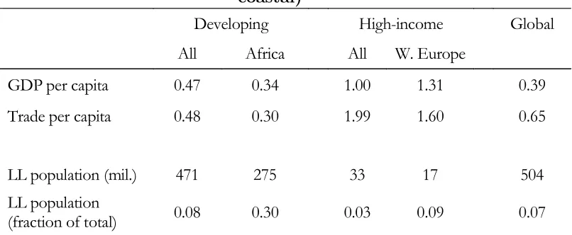
The analysis is particularly relevant to Africa, a continent of histori-cally low growth and still home to the majority of the world’s very poorest
countries. With a third of the population being landlocked, and manufac-turing centres continuing to agglomerate in East Asia, penetrating global markets may be unrealistic in the near-term (Radelet & Sachs 1998, Col-lier 2008). As a result, African economic integration is now a top priority of donors and policy makers. The African Development Bank for example has a dedicated Regional Integration & Trade Division, and in November
2014 approved a new Regional Integration Policy and Strategy for 2014-2023.7 For the landlocked in particular, Collier and O’Connell (2007) argue
that "the most obvious growth strategy for such a country is to service the markets of its neighbours" (p.38).
The results here show that reducing trade costs enables a country to pursue such a growth strategy. In particular, reducing trade costs increases
IMA and so increases the spillover of neighbouring growth into domestic growth. Based on the gravity results, I can quantify the extent to which speci…c policies will increase IMA, and so ultimately estimate the impact of such policies on output and growth. To demonstrate this, I consider a speci…c policy currently under review: an extension of the West African
6Over the period studied for example, the coe¢ cient of variation (the standard
devi-ation divided by the mean) of real GDP was 0.27 in Sub-Saharan Africa, 0.18 globally and 0.13 in the OECD (based on World Bank WDI …gures). Further, 7 Sub-Saharan African countries witnessed a swing in real GDP of over 25 percent from one year to the next at some point during the period.
7The President of the Bank recently listed his top priorities for the continent as
currency union to include six additional countries. I estimate that such a policy could increase aggregate West African output by around 40 percent,
with substantially larger gains for non-members of the existing currency union. Quantifying the (trade-related) gains from such policies can assist policy makers in evaluating expected gains against potential losses (for the currency union case see Santos Silva and Tenreyro 2010 for a discussion).
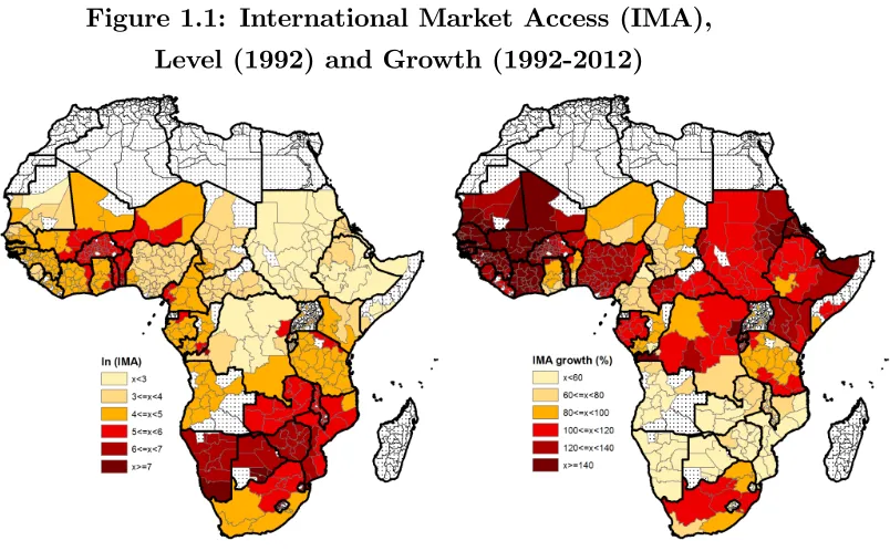
Figure 1.1 demonstrates the variation in IMA, and its growth, over the period. The regions bordering South Africa and Nigeria bene…t from the
highest levels of IMA (left-hand map), although growth has been strongest in the far western regions (right-hand map). As a calibration exercise, I document the importance of South Africa and Nigeria –together accounting for half of African GDP –to their immediate neighbours. Due to its impact on IMA, I …nd that each additional percentage point of growth in South Africa is re‡ected in at least half a percentage point of growth in each
Figure 1.1: International Market Access (IMA),
Level (1992) and Growth (1992-2012)
The paper proceeds as follows. Section 1.2 presents the trade model that derives domestic output as a function of market access. Building on this, Section 1.3 presents the empirical framework which proceeds in two stages. First, a gravity model is used to estimate the IMA term. Second, regional output is regressed on this market access term, generating my main results
of interest. Section 1.4 discusses the data, in particular the luminosity data and construction of regional output. Section 1.5 presents the results and Section 1.6 considers the growth and policy implications. Section 1.7 concludes.
1.2
Theory
each region j is weighted by the level of competition for that region, the cost of trading with regioni and the elasticity of trade w.r.t. trade costs.
There are many regions, indexed by i when the origin of an export and
j when the destination. Regions produce a continuum of goods (indexed bys) using a Cobb-Douglas technology with labour and capital as inputs. The marginal cost of producing a good of varietys in region i is given by:
M Ci(s) =
wir1 zi(s)
(1)
where wi is the wage rate, r is the capital rental rate and zi(s) is the
e¢ ciency with which regioni can produce varietys.8 Following Eaton and
Kortum (2002), e¢ ciency zi(s) is stochastic, and drawn from an extreme
value distribution given by Fi(z) = e Tiz with Ti > 0 and > 1. The
parameterTiincreases the mean of the distribution, meaning thatTi can be
interpreted as regioni’s level of technology (as average e¢ ciency is higher). A lower increases the variability of the distribution, such that i will be more e¢ cient in the production of some goods than others. As noted by Eaton and Kortum,Ti is therefore a source of absolute advantage for region
i, and is a source of comparative advantage.
If labour is mobile, utility levels must be constant across regions in
equilibrium:
U = wi
Pi
(2)
where U is the constant level of utility across regions and Pi is the
consumer price index in region i.9 Crucially, trading goods across regions
is costly. Modelling trade costs using the standard iceberg approach, the price of a good produced in regioniand sold in regionj is given bypij(s) = ijpii(s) where ij 1 is the trade cost and pii(s) is the price of the good
sold locally. Regionisuppliesj with goods if it is the lowest cost supplier,
and so in general,j sources all its goods from the regions from which it can achieve the lowest price.
The expression for the overall price indexPi in regioniis solved
explic-itly in Eaton and Kortum (2002), and is given by:
Pi =a1
X
j
Tjwj ij (3)
wherea1 is a constant. Following Donaldson and Hornbeck (2013), this
expression can be termed "consumer market access" (CMA), as it captures the access of consumers ini to goods produced elsewhere, with prices in i
increasing in the trade cost ij. A further expression derived explicitly in
Eaton and Kortum (2002) is a gravity equation giving the value of exports (Xij) fromi toj:
Xij =a2Tiwi ij PjYj (4)
where a2 is a constant and Yj is the income of region j. Intuitively,
i supplies j with the goods for which it is the lowest cost supplier. The likelihood of being this low cost supplier increases ini’s level of technology
Ti and the overall price level Pj (where a higher price level corresponds to
less competition for market j). Higher income Yj boosts the overall level
of demand coming fromj. The opposing force is the trade cost ij, which
reduces i’s competitiveness in region j. It can also be seen in (4) that captures the elasticity of trade w.r.t. trade costs. This is consistent with
the earlier interpretation of as the source of comparative advantage: as comparative advantage weakens (higher ), the importance of geographic barriers increases.10
As an accounting identity, the output Yi of region i is the sum of its
10Technically, a higher reduces the likelihood of outliers in the e¢ ciency distribution
Fi(z)that enableito produce goodscheaply enough to overcome geographic obstacles
exports to all regions j,
Yi =
X
j
Xij (5)
where PjXij includes Xii (i.e. local consumption). Substituting for
Xij from the gravity equation (4), and replacing Pj and wi from (3) and
(2) respectively, we can derive an expression for the output of regioni as a weighted product of the output of all regionsj:
Yi =a2TiU Pi
X
j
ij CM A
1
j Yj (6)
where Pj ij CM Aj1Yj is the "…rm market access" (FMA) of region
i. This expression shows that the output of region i is increasing in its access to the markets of all regions j: other things equal, output is higher in regions with cheap access ( ij ) to large markets (Yj) that have limited
sources of cheap supply from elsewhere (CM Aj1). To see this explicitly, we can take logs of equation (6) to arrive at:
ln(Yi) = a3+ ln(Ti) + ln(CM Ai) + ln(F M Ai) (7)
wherea3is just a constant given byln(a2) ln(U)and I use the result
that Pi CM Ai.
Donaldson and Hornbeck (2013) show that asF M Ai =Pj ij CM A 1 j Yj
and CM Aj =
P
i ij F M A 1
i Yi, any solution to these two equations must
satisfy F M Ai = CM Ai. That is, the two measures of market access are
in fact the same. Substituting this into equation (7), we get a model for the output of region i as a simple log-linear function of its market access (M Ai):
ln(Yi) = a3+ ln(Ti) + (1 + ) ln(M Ai) (8)
where M Ai =Pj ij Yj
M Aj .
output increases log-linearly in market access. Market access is the sum of output in all regions j, each Yj being weighted by (i) the cost of trading
with i, and (ii) j’s own market access M Aj. This second term captures
the degree of competition for marketj: ifj itself has strong market access, then a smaller share of its imports are sourced fromiand hence increases in import demand (coming from increases inYj) are muted. Given a panel of
observations on regional output, equation (8) therefore provides a testable prediction for the empirical analysis.
1.2.1 Discussion: Mobile labour
The assumption of mobile labour may seem strong in the context of an
international trade model. It is used here only to simplify the derivations however; Alder (2015) works with the same underlying model, except that he assumes immobile labour, and notes that "both versions of the model lead to a log-linear relationship between income and market access. The di¤erence is the predicted elasticity, but this is estimated from the data" (p.22). In this paper I also estimate the predicted elasticity from the data,
and use the model for its qualitative prediction of a log-linear relationship between output and market access. Hence the assumption of mobile labour does not a¤ect the empirical approach that follows.
Unlike Alder (2015) and Donaldson and Hornbeck (2013) however, both of which work in the context of intra-country trade, this paper is primarily
interested in inter-country trade. In the model and the empirical work, intra-country dynamics are ultimately overlooked. (The model itself does not distinguish between domestic and foreign regions, although when it is adapted for the empirical framework, domestic regions are omitted in the calculation of market access.) The paper considers the relative response of domestic regions to changes in their IMA; if there is a shock to a particular
To capture these dynamics completely, a mixed regional/international model would be required. Although that exercise is not undertaken here,
it is useful to think through the implications qualitatively. Suppose a par-ticular region receives a boost to its IMA due to growth in a nearby region across the border. This not only increases export demand, it also reduces the domestic region’s price index; an increase in foreign output Yj works
in the same direction as a fall in trade costs.11 This fall in the price level
temporarily increases the real wage, leading to in-migration. (It is assumed
that workers move wherever the real wage is highest, hence the need for a constant real wage in equilibrium.) As the region’s workforce increases how-ever, the nominal wage falls due to diminishing returns to labour. Migration therefore restores the domestic equilibrium, but the region that received the initial (positive) IMA shock received an additional output boost due to in-ternal migration.12 If I was to model internal dynamics explicitly, it is
therefore likely that it would reinforce the predictions of the model above. In particular, even if I were to assume immobile labour between domestic and foreign regions, but mobile labour between domestic regions, the model should still predict a positive relationship between output and IMA.
1.3
Empirical Framework
The model has a strong intuitive appeal: higher market access attracts both …rms - seeking cheap access to sources of demand - and consumers - seeking cheap access to goods. To implement the model empirically however, there are a number of challenges. Firstly, the market access term from
equa-tion (8) includes domestic output, as it is a weighted sum of the output in all regions j. This creates a clear endogeneity problem, and would
re-11From equation (3), the price index (P
i) is inversely proportional to consumer market
access. A fall in trade costs and an increase in foreign output both increase consumer market access, and hence reduce the price index
12See Overman et al. (2010) for a more detailed discussion of the spatial implications
quire estimates of internal trade costs ii in order to be implemented. A partial solution to the problem, pursued by Redding and Venables (2004)
and Mayer (2009), is to estimate internal trade costs and run the model with both "domestic" and "foreign" market access terms. An alternative approach, also pursued by Mayer (2009) and by Donaldson and Hornbeck (2013), is to drop the inclusion of domestic output from the market access term.13 As I am interested in international spillovers, this is the approach
I follow here. Indeed, to concentrate on international spillovers, I include
only foreign regions in the calculation of M Ai. I term this "international
market access" and denote it byIM Ai.14
Secondly, equation (8) remains an implicit function of Yi even when
domestic regions are excluded from the calculation of market access. This is due to theM Ajterm in the denominator, which accounts for the degree of
competition for the importing regionj. Following Donaldson and Hornbeck (2013), I therefore approximate the theoretically correct market access term with a simpler expression given by M Ai =
P
j ij Yj. As noted by the
authors, the two market access terms are highly correlated in practice but the approximation does not require each market access term to be explicitly derived from the model.15 As I work with international market access, my
13Redding and Venables (2004) outline a similar trade model to the one presented
here but with immobile labour. Their model derives the wage rate in countryi(wi) as
a log-linear function of the country’s market access. They use income per capita as a proxy for wi and consider various approximations to calculate internal trade costs ii
for the (domestic) market access term. Mayer (2009) extends the Redding and Venables approach to a panel setting. He presents empirical results both with approximations for
ii, and with domestic output dropped from the market access term. Both approaches
show strongly signi…cant e¤ects of market access on domestic income per capita.
14This is consistent with my approach of using cross-country gravity regressions to
estimate the trade cost function (below), and I show in robustness checks that my results also hold when domestic regions are included in the market access term.
15That is, eachM A
i term could be derived fromM Ai=Pj ij Yj
M Aj as this is a system
variable of interest is therefore given byIM Ai =Pj2F ij Yj
M Aj P
j2F ij Yj,
whereF denotes the set of foreign regions.
Allowing for randomness in the data and adding a time dimension, equa-tion (8) therefore suggests the following speci…caequa-tion:
ln(Yit) = '0+'1ln(IM Ait) + i+ ct+ it (9)
where '0 is a constant, Yit is the output of regioni in year t, IM Ait =
P
j2F ij Yjt, iand ct are region and country-year …xed e¤ects respectively
(to control for the productivityTi of regioni) and it is an error term.
Without information on trade costs ij and the elasticity of trade w.r.t.
trade costs ( ), equation (9) cannot be estimated directly. As an initial
step in the empirical work, and departing from Donaldson and Hornbeck (2013), I therefore apply a gravity model to estimate these values.16 To generate my main results of interest, I then regress regional output Yit on
the estimated market access termIM A[it.
1.3.1 Gravity: constructing IM A[it
As noted by Anderson and van Wincoop (2004), the trade cost ij is
typi-cally assumed to be multiplicatively separable in its factors, such that:
ij = M
Y
m=1
(zijm) m (10)
where zij = z1ij ::: zijm ::: zMij is the vector of trade cost factors
between i and j (e.g. distance, shared language) and m is the elasticity
of ij w.r.t. factor m. Substituting this expression into the international
16For the trade cost
ijDonaldson and Hornbeck use historical transport cost estimates
market access term, we have:
IM Ai =
X
j2F
" M Y
m=1
(zijm) m #
Yj (11)
and from the gravity equation (4) we can get consistent estimates of the
m terms by running the following regression:17
ln(Xij) = 0 ln( ij) + i+ j + ij (12)
= 0 X
m
m ln(z m
ij) + i + j+ ij
where 0 is a constant and ij is the error term. That is, if we observed
trade ‡ows between i and j; we could consistently estimate international market access. Although I do not have regional trade data, I can estimate (12) at the country level. A single year of trade data would su¢ ce for consis-tency, however I include the full set of trade observations over 1992-2012 for greater e¢ ciency. As trade cost factors (zij) I include distance, a contiguity
dummy, common language dummy, regional trade agreement (RTA) and
currency union (CU) dummies (Mayer 2009, Head and Mayer 2015). The estimated coe¢ cients allow me to construct international market access as:
[ IM Ait =
X
j2F
" M Y
m=1
(zijm) dm #
Yjt (13)
where the dm terms are the estimated coe¢ cients from (12).
Taking a simple example to clarify this procedure, suppose that the only relevant trade cost is the distance between i and j. In this case, we have ij = distij from equation (10) and ln(Xij) = 0 ln(distij) + i+ j+ ij from the gravity equation (12). Suppose that from the gravity
equation we estimate c = 1:1, the mean estimate from Head and Mayer
17The exporter and importer …xed e¤ects
iand j control for theln(Ti), ln(U Pi),
(2015). Then from equation (13) the market access term would be given by
[
IM Ait=Pj2F distij1:1Yjt. This example highlights that the market access
term used here is a more general form of the well-known Harris (1954) "market potential" term given byM Pit =
P
j Yjt
distij.
1.3.2 Regional output and market access
Having constructed my market access term, I can turn to my primary ques-tion of interest: how do changes in internaques-tional market access a¤ect do-mestic (regional) output? To do so, I run the following regression based on (9):
ln(Yit) = 0+ 1ln(IM A[it) + i+ ct+"it (14)
whereIM A[it is from (13). In alternate speci…cations I will also include
a region-speci…c linear time trend, to allow for di¤erent growth paths of the regions.
1.3.3 Discussion: Empirical Strategy
To clarify the empirical strategy, equation (14) is the main regression of
interest, and is estimated across a panel of sub-national regions over 1992-2012. In order to estimate (14) however, we require estimates of the elastic-ity of trade w.r.t. trade costs ( ) to create theIM A[it term. In the absence
of region-level trade data, is therefore estimated by a gravity regression at the country level - given by equation (12).
[
IM Ait is the sum of output in all foreign regions, with each region
weighted by the cost of trade with the domestic region. The cost of trade is assumed to be …xed, and so changes in IM A[it are driven exclusively by
country that have cheaper access to foreign African markets respond more to output changes in those markets than regions within the same country
that have more costly access.
To implement this strategy, equation (14) includes both region and country-year …xed e¤ects. The region …xed e¤ects control for time-invariant factors that could induce a spurious correlation between market access and regional output in the cross-section. In Africa, prominent among such fac-tors are the disease environment and physical geography. The country-year
…xed e¤ects control for political and macroeconomic shocks. Such shocks have been frequent and severe in Africa in the recent past: during the period studied for example, 7 African countries witnessed a swing in real GDP of over 25 percent from the previous year. In the presence of these dramatic macro shocks, it is di¢ cult to identify international growth correlations or spillovers when working with country-level data. Zimbabwe is a notable
ex-ample: between 2002 and 2008, it su¤ered an overall decline in real GDP of 31 percent, whilst each of its neighbours posted positive growth rates each year. This does not mean that Zimbabwe did not bene…t from its neigh-bours’growth, rather that the domestic macro policies were so disastrous as to completely o¤set such bene…ts. Analysing regions within countries there-fore allows for a cleaner identi…cation of growth spillovers across countries
by controlling for these political and macro shocks.
A limitation of the approach however is that African GDP (and therefore market access) has been growing over time, and so other factors that are also growing over time could drive a correlation between market access and output. The country-year …xed e¤ects control for those factors that a¤ect
access is more heavily in‡uenced by other hinterland regions just across the border). Although it is not possible to control for such issues completely, it
is noted that lights did not grow signi…cantly faster on average in hinterland regions than capital regions over the period considered here.18 Henderson et al. (2012) …nd a slightly higher increase in lights growth in hinterland areas of Africa than large cities, although they note that such a di¤erence is extremely small. My preferred set of results also include region-speci…c time trends, so that I am testing to what extent a region’s lights output
deviates from trend in response to changes in market access.
1.4
Data
1.4.1 Bilateral trade ‡ows
I construct a panel of bilateral imports using data from the UN Comtrade
Database.19 The dependent variable is the value of imports of country i
from countryj in year t. The independent variables - the distance between countries i and j (denoted distij, measured in km), contiguity (denoted
border), language, CU and RTA dummies - are all taken from the gravity database of Head et al. (2010), available at http://www.cepii.fr/.
1.4.2 Lights data
I exploit luminosity data to create a balanced panel of sub-national regional output over 1992-2012. Described in detail in Henderson et al. (2012), night time light readings have been recorded by the U.S. Defense Meteorological
Satellite Program (DMSP) since the 1960s, with a public digital archive beginning in 1992. Before being publicly released, the data are processed to remove most natural sources of light, including moonlight, sunlight, auroral
18I denote a "capital region" here as the largest region in each country based on lights
output in 2000. Lights output grew in capital regions by 5 percent per year on average. In all other regions, they grew by 4 percent per year on average.
19I work with import reports as these are known to be more reliable than export
activity and forest …res. The remaining lights are largely arti…cial, re‡ecting the use of energy for both consumption and investment purposes. Lights
data therefore enable economic activity to be tracked at a local level, where o¢ cial statistics are either unreliable or non-existent.
Light intensity is provided at the pixel-level, with each 30-arcsecond pixel given an integer light reading between 0 and 63.20 Constraining light
readings to fall within this range re‡ects the available sensor technology, and in the African case many pixel-year observations omit no recorded light (an
issue known as "bottom coding"). There is likely in practice to be some limited activity in such areas, not generating enough light to be captured by the sensors. To check that this is not a¤ecting the main results, I show in the Appendix that the results are robust to restricting the sample to areas that have recorded light readings in every year, as well as dropping 1992 from the sample.21 Following standard practice (Henderson et al. 2012,
Storeygard 2014), I calculate a simple average of light readings for years in which there is more than one satellite. Doing so provides a pixel-year panel of light readings for the entire continent.
As the pixels are so small, I need to aggregate them into economically-meaningful units. I aggregate to administrative level 1 regional units (herein "Admin 1 regions"), with GIS boundaries provided by Natural Earth.
Fig-ure A1 in the Appendix provides a map of the regional boundaries. The use of Admin 1 regions provides adequate within-country variation, whilst ensuring that the model remains plausible and tractable.
Prior to aggregating, I clean the raw lights data by making use of the "ur-ban extents" dataset provided by the Global Rural Ur"ur-ban Mapping Project
(GRUMP).22The GRUMP dataset classi…es the globe into areas of "urban"
20A 30-arcsecond pixel has an area of approx. 0.86 square km at the equator.
21There is an abnormally large proportion of observations with a light reading of zero
in 1992. Thirty percent of regions have a light reading of zero in 1992, dropping to 20 percent in 1993 and falling gradually to 7 percent by 2012.
22Center for International Earth Science Information Network - CIESIN - Columbia
and "rural", also at a spatial resolution of 30-arcseconds. The classi…cation of an urban area is based on population estimates; contiguous urban
ar-eas should consist of at lar-east 5,000 persons.23 In aggregating to Admin 1 regions, I sum only across lights in urban areas. Doing so enables me to include only areas where people actually live and economic activity takes place, excluding extremely small settlements and random noise in the data (such as lights from gas ‡ares and lights that spill across borders).24 A
further advantage is that I can always classify contiguous urban cells,
es-sentially the same city, as belonging to the same region.25
Lights and economic output
As discussed in Pinkovsky (2013), a number of empirical papers have now used luminosity data as a proxy for output. The …rst paper to investigate
this relationship systematically was Henderson et al. (2012), who demon-strated a robust correlation between luminosity readings and o¢ cial GDP estimates in a panel of countries. The authors show that this relationship holds both with and without a country time-trend, and also when esti-mated in "long di¤erences". Their baseline results suggest an elasticity of real GDP w.r.t. lights of around 0.3.
Rural-Urban Mapping Project, Version 1 (GRUMPv1): Urban Extents Grid.
Palisades, NY: NASA Socioeconomic Data and Applications Center (SEDAC). http://dx.doi.org/10.7927/H4GH9FVG accessed 28/10/2014. See also Balk et al (2006).
23CIESIN also provide a "settlement points" dataset, which provides coordinates of
known settlements of over 1,000 persons. Each urban extent should therefore correspond to at least one settlement point (due to the higher populaton threshold). I drop any contiguous urban extent pixels that do not have a settlement point associated with them. This also ensures that any foreign urban areas that spill across the border are not (incorrectly) included in a domestic region.
24Indeed, my approach shows a substantial and signi…cant correlation between the
regional lights data and o¢ cial GDP estimates on the South African sub-sample below. Simply aggregating across lights within regions does not (even nearly) pass this "sense check".
25I take the centroid of each contiguous block and assign the region according to the
The principal advantage of using lights is that they enable estimates of economic activity in local areas for which o¢ cial …gures are unavailable.
In Africa, Michalopoulos and Papaioannou (2013) use luminosity data as a proxy for income per capita across ethnic territories. To justify this, they …rst show that across di¤erent "enumeration areas" (typically villages or small towns), lights output is highly correlated with a wealth index created using Demographic and Health Surveys data. More recently, Storeygard (2014) uses lights output as a measure of city-level output across a number
of African countries. He tests that light output approximates o¢ cial GDP at the sub-national level by running regressions of GDP on luminosity for Chinese prefectures (over 1992-2005) and South African magisterial districts (over 1996-2001). The relationship is highly signi…cant in both cases, with elasticities in the range 0.2 to 0.3.
Following these previous papers, I also test to what extent the luminosity
data used here correlates with o¢ cial GDP …gures. Figure A2 provides a visual illustration, plotting the light output of Rwanda - a country that has grown steadily since the late-1990s, and Zimbabwe - a country where output has declined slightly over the period.26 The contrast is clear from the lights
output, with growth in Rwanda notable in all areas of the country. To check the correlation between GDP and lights explicitly, I sum the regional lights
…gures above within each country, and run the following regression (as in Henderson et al. 2012):
ln(zct) = ln(yct) + c+ t+wct+ ct (15)
where zct is the real GDP of country cin year t (from the World Bank
World Development Indicators),yct is the light reading of countrycin year
t, c and t are country and year …xed e¤ects respectively, wct is a
lin-ear country time-trend, and ct is an error term. The regression is run
26Output in Rwanda declined by around 50% as a result of the genocide in 1994, and
at country-level due to the paucity of African GDP estimates at the sub-national level (which is the primary motivation for using lights). However,
Statistics South Africa have been producing annual GDP estimates for Ad-min 1 regions since 1995, and so I am able to run the regression at the regional level on this small sub-sample.
Results are provided in Table 1.1. Columns (1) and (2) are run at the country-level over 1992-2012, and columns (3) and (4) are run for the South African regions over 1995-2012. Columns (2) and (4) include the
linear time trendwct, and thus measure correlations in terms of deviations
from trend. All columns indicate a signi…cant correlation between o¢ cial GDP and lights, with an elasticity of around 0.5 when the time trend is excluded. The level of signi…cance is somewhat weaker when using the South African regional data, although with such a limited sample the results are encouraging.
Table 1.1: The elasticity of GDP w.r.t. lights SAF (regions)
(1) (2) (3) (4)
ln(yct) 0.506*** 0.329*** 0.468* 0.145*
(0.059) (0.070) (0.229) (0.073)
Time trend No Yes No Yes
Obs. 819 819 162 162
Countries/Regions 39 39 9 9
R-Squared 0.83 0.94 0.58 0.76
Robust standard errors (clustered by country) in parentheses.
***p <0.01, **p <0.05, *p <0.1
at the local level in Africa. This justi…es the use of lights as a proxy for regional output in the estimation of equation (14). Ultimately however,
I would like to use the results of (14) to make inferences regarding the response of domestic output to changes in foreign output. That is, I am ultimately interested in the response of GDP in region i (denoted zi) to
changes in GDP in regionj (denotedzj), rather than the response oflights
ini (denotedyi) to lights in j (denotedyj).
It can be shown that the two elasticities are the same. Denote the
"GDP elasticity" by "1 dzdzij zj
zi and the "lights elasticity" by "2
dyi
dyj
yj
yi. We have also estimated the elasticity of GDP to lights in Table 1.1, denoted by"3 dzdyiiyzii. From the chain rule, dzdzji = dzdyiidydyij
dyj
dzj and so, multiplying by
zj
zi,
"1 = dzi
dzj
zj
zi
= dzi
dyi
yi
zi
| {z }
"3
dyi
dyj
yj
yi
| {z }
"2
dyj
dzj
zj
yj
| {z }
"31
= "2:
I use this result in section 1.6 to analyse the implications of changes in IMA for changes in domestic output.
Issues and limitations
As discussed in Michalopoulos and Papaioannou (2013), luminosity data su¤ers from saturation and "blooming". Saturation occurs due to the sen-sor technology, which only registers light output up to a certain level. This
African sample less than 0.0001 percent of pixels are top-coded.
A more pertinent issue with the lights data is "blooming" or "overglow".
Blooming occurs when a source of light is bright enough that some of its glare is captured in the readings of neighbouring pixels. This is a geocoding error, that could generate a manual correlation between lights growth in neighbouring areas. Reassuringly however, Michalopoulos and Papaioannou (2013) …nd that because luminosity is generally low in Africa, blooming is not a major concern in this sample. More concretely, Pinkovsky (2013)
…nds that the e¤ect of blooming on measured light output is insigni…cant beyond a 10 km bu¤er. For my baseline results, I therefore bu¤er all country borders by 10 km to account for blooming.27
1.4.3 Market access
To construct the IM A[it term, I calculate the distance from each region i
to each foreign regionj. Distances are calculated using the great circle dis-tance from the largest city in each region, based on lights output in 2000.28
In calculating IM A[it, I restrict the set of foreign regions j to lie within
the same UNECA "sub-region" as i - these consist of West Africa, Cen-tral Africa, Eastern Africa and Southern Africa.29 The motivation for this
is that (i) the vast majority of international trade takes place within the same sub-region, and (ii) when considering trade ‡ows across sub-regions,
27Because borders are bu¤ered by 10 km on each side, there is a minimum of 20 km
between light readings either side of country borders. In practice, bu¤ering country borders makes very little di¤erence to the results. In the Appendix I show that my results are almost identical if no bu¤er is used, and I have also experimented with other bu¤er distances, again with very little e¤ect.
28I take the centroid of the largest city (contiguous block of urban cells) based on
light output in 2000. To accurately calculate distance, I then project these points to the African Sinusoidal (projected) coordinate system. Geodesic distances, that take into account the curvature of the globe, are then calculated using the Generate Near Table tool. All steps are done in ArcMap 10.2.1.
29See http://www.uneca.org/pages/subregional-o¢ ces. The Admin 1 regions of any
the relative locations of regions within the same country becomes trivial relative to the overall distance between domestic and foreign regions.
Run-ning equation (14) including twoIM A[it terms, one calculated from foreign
regions within the same UNECA sub-region as i, and one calculated from foreign regions outside the UNECA sub-region, shows that only the …rst is signi…cant. In addition, the main results of interest (presented in Table 1.4) remain strongly signi…cant if IM A[it is calculated using all foreign regions.
For the baseline results in Table 1.4, I exclude all observations from
countries that are in con‡ict according to the UCDP/PRIO Armed Con‡ict Database.30 Con‡icts tend to be concentrated in particular regions within a
country, and so some regions su¤er large falls in output regardless of changes in their market access. It therefore seems sensible to exclude all regions of a country for years in which the country is in con‡ict. In Appendix A.2 I show that the results are robust to including all observations, including
con‡ict years.
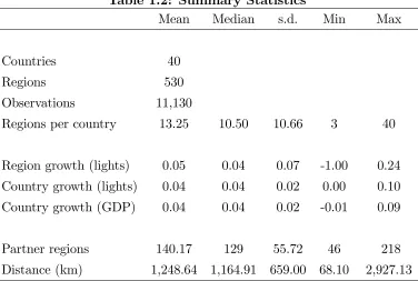
Summary statistics are shown in Table 1.2. As the lights data are avail-able over 1992-2012, the summary statistics and all subsequent analysis covers this period. All mainland Sub-Saharan African countries are in-cluded except for Equatorial Guinea, which is dropped (as in Henderson et al. 2012) because almost all of the light output is from gas ‡ares. As a tiny
country, it also has only one mainland region.
30Only "intense" con‡ict years are excluded, which are those that result in a minimum
Table 1.2: Summary Statistics
Mean Median s.d. Min Max
Countries 40
Regions 530
Observations 11,130
Regions per country 13.25 10.50 10.66 3 40
Region growth (lights) 0.05 0.04 0.07 -1.00 0.24
Country growth (lights) 0.04 0.04 0.02 0.00 0.10 Country growth (GDP) 0.04 0.04 0.02 -0.01 0.09
Partner regions 140.17 129 55.72 46 218 Distance (km) 1,248.64 1,164.91 659.00 68.10 2,927.13
Growth rates are compound annual averages, and must be multiplied by 100 for a percentage …gure.
1.5
Results
1.5.1 Gravity model
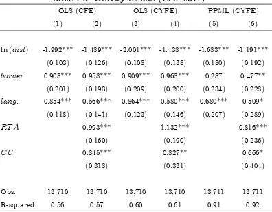
Table 1.3 presents the results of running equation (12), a structural grav-ity model, for the Sub-Saharan African sample over 1992-2012. The set of control variables follows Mayer (2009), and consists of distance (km), contiguity (denotedborder), common language, RTA membership and CU membership. This is a standard set of controls in the gravity literature (see e.g. Head and Mayer 2015), although in alternate columns I exclude the
(Santos Silva and Tenreyro 2006) instead of ordinary least squares (OLS). The variables enter signi…cantly throughout, with each taking the
ex-pected sign. Perhaps the most striking results are the magnitudes of the distance and RTA variables. Although estimates of RTA e¤ects vary widely, Head and Mayer’s (2015) meta-analysis …nds a median estimate of just 0.28. The large coe¢ cients in Table 1.3 are particularly surprising given the com-mon view that African RTAs are less e¤ective than average (see e.g. Roberts and Deichmann 2011). A satisfactory explanation for this …nding would
re-quire further research, although I note here that the main results of interest for this paper - the impact of market access on output - are not sensitive to the particular coe¢ cients in Table 1.3.31
As with the RTA dummy, the coe¢ cient on distance in the OLS regres-sions is slightly larger than typical estimates.32 This is less surprising than
the RTA e¤ect however, as the poor state of African infrastructure (Limao
and Venables 2001) and logistics services (Arvis et al. 2012) both sug-gest that transport costs rise rapidly with distance. In practice, it is likely that African trade is even more geographically concentrated than the esti-mates here suggest. Survey evidence shows that informal cross-border trade occurs on a substantial scale across the continent, with volumes in some ar-eas comparable to o¢ cial trade (Lesser & Moisé-Leeman 2009, Afrika and
Ajumbo 2012). Much of this trade is in food, agriculture and low quality manufactures, meaning that much of it is concentrated around border re-gions (Lesser and Moisé-Leeman 2009, Golub (forthcoming)). Hence overall trade likely declines more rapidly in distance than o¢ cial trade: the esti-mates here may in fact underestimate the true e¤ect of distance on trade in Africa.
31In Table 1.4 I show that the e¤ect of market access on output is robust to the
di¤erent gravity speci…cations in Table 1.3, and in robustness checks I show that this further extends to using the median gravity estimates from Head and Mayer (2015).
32Head and Mayer (2015) …nd a median coe¢ cient on distance of -1.1 from structural
Table 1.3: Gravity results (1992-2012)
OLS (CFE) OLS (CYFE) PPML (CYFE)
(1) (2) (3) (4) (5) (6)
ln (dist) -1.992*** -1.489*** -2.001*** -1.438*** -1.683*** -1.191*** (0.103) (0.126) (0.108) (0.138) (0.180) (0.192)
border 0.908*** 0.958*** 0.909*** 0.968*** 0.287 0.477**
(0.201) (0.193) (0.209) (0.200) (0.234) (0.228)
lang: 0.854*** 0.566*** 0.864*** 0.580*** 0.680*** 0.509*
(0.118) (0.141) (0.123) (0.146) (0.207) (0.289)
RT A 0.993*** 1.132*** 0.816***
(0.160) (0.190) (0.236)
CU 0.845*** 0.827** 0.666*
(0.318) (0.331) (0.404)
Obs. 13,710 13,710 13,710 13,710 13,711 13,711
R-squared 0.56 0.57 0.60 0.61 0.91 0.92
Robust standard errors (clustered by country) in parentheses. *** p<0.01, ** p<0.05, * p<0.1
1.5.2 Regional output and market access
Having generated estimates for the trade cost parameters, I can now con-sider the e¤ect of IMA on regional output. To do so I substitute the coef-…cients from Table 1.3 into my expression for market access, IM A[it from
equation (13), and regress regional output on this estimated market access
term - equation (14).
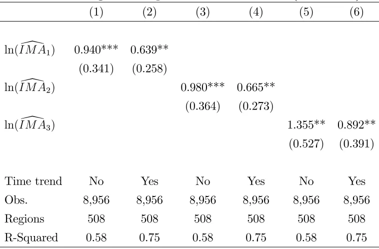
The results from equation (14) are presented in Table 1.4. I consider three alternative estimates of market access: IM A[1 is calculated using
col-umn (2) from Table 1.3, IM A[2 uses column (4) from Table 1.3 and IM A[3
uses column (6) from Table 1.3. That is, the di¤erent market access terms
speci…ca-tions in Table 1.3: OLS (CFE), OLS (CYFE) and Poisson (CYFE). In all columns of Table 1.4, IMA has a positive and highly signi…cant
e¤ect on regional output. I consider the results in columns (4) and (6) to be the best estimates, and will work with these estimates in the calibration below. In both cases the parameters of theIM A[ term are estimated using a full set of CYFE, and any long-term regional growth paths are controlled for with the time trend. These estimates put the elasticity of regional output w.r.t. IMA in the range 0.7 to 0.9.
These estimates suggest that regional output responds strongly to changes in IMA. Previous work, estimated at country-level, has produced compa-rable albeit slightly smaller estimates. Mayer (2009) regresses income per capita on a measure of "foreign market potential" over 1960-2003, …nding an elasticity of 0.88 from a random e¤ects model and 0.57 when including country …xed e¤ects.33 In earlier work, Redding and Venables (2004) apply
the same approach as Mayer on a single cross-section of countries in 1996, and …nd an elasticity of 0.48 on "foreign market access".
33Mayer’s (2009) "foreign market potential" term is, from his model, very similar to
Table 1.4: Regional output and market access (1992-2012)
(1) (2) (3) (4) (5) (6)
ln(IM A[1) 0.940*** 0.639**
(0.341) (0.258)
ln(IM A[2) 0.980*** 0.665**
(0.364) (0.273)
ln(IM A[3) 1.355** 0.892**
(0.527) (0.391)
Time trend No Yes No Yes No Yes
Obs. 8,956 8,956 8,956 8,956 8,956 8,956
Regions 508 508 508 508 508 508
R-Squared 0.58 0.75 0.58 0.75 0.58 0.75
Robust standard errors (clustered by region) in parentheses. *** p<0.01, ** p<0.05, * p<0.1
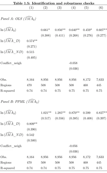
1.5.3 Identi…cation and robustness
The results presented in Table 1.4 show that there is a robust correlation
between changes in a region’s IMA and changes in its own output. Based on the model presented in Section 1.2, I argue that this is driven by trade: as IMA increases, demand for local goods increases which drives increases in local production. In this sub-section I aim to establish both that trade is indeed the driving mechanism, and that this is a causal relationship. To do so, I present a number of falsi…cation and robustness checks in Table 1.5.34
Firstly, if the e¤ect of IMA is working through trade, we would ex-pect to …nd a smaller e¤ect between countries that do not have trading relationships with each other.35 To test this, I gather data on diplomatic
34Each column in Table 1.5 includes the region-speci…c linear time trend.
35The e¤ect would not necessarily be zero, as informal cross-border trade takes place
relations from the Correlates of War’sDiplomatic Exchange Database, and classify countries based on whether they had diplomatic relations with each
other over the period (1992-2012). For each region, I then calculate two
[
IM A terms: one across countries with which it had diplomatic relations (IM A[_D), and another across regions in countries with which it did not (IM A[_N D). Reassuringly, in column (1) we see that the IM A[ term is signi…cant only amongst countries with diplomatic relations.
Secondly, there may be localised shocks, such as higher commodity prices
or cross-border investment projects, that simultaneously bene…t neighbour-ing regions. This would generate a positive correlation between output and market access, but not due to the trade channel posited here. To reduce such concerns, column (2) excludes all regions within 100 km of the domes-tic region when calculating IM A[.36 Column (3) drops the closest foreign
region, so that any localised shock would have to cover a number of regions
to drive the correlation between IMA and domestic output. In both cases, theIM A[ term remains highly signi…cant.
Column (4) controls for neighbouring con‡icts, which can spill across national borders through refugee ‡ows, direct violence or destruction of infrastructure. This acts like a speci…c localised shock, generating a simul-taneous (negative) shock to both IMA and domestic output. To control
for this, I create a dummy variable (denoted conf lict_neigh) that equals 1 if a region’s nearest neighbour is in con‡ict in year t.37 In column (4)
this variable enters negatively but insigni…cantly, whereas the coe¢ cient on
[
IM A remains largely unchanged and highly signi…cant.
Finally, columns (5) and (6) address potential reverse causality from
do-mestic output to IMA. This occurs because an increase in dodo-mestic output increases every foreign region’s IMA, increasing their output, which in turn increases the domestic region’s IMA. In practice this concern is reduced
36That is 100 km between the "capital" of each region.
37Neighbouring con‡icts are de…ned in the same way as domestic con‡icts (Section
because every region’s IMA is calculated based on the output of a large number of regions (140 on average, see Table 1.2). Still, it may be the
case that some regions are large enough to individually a¤ect output in the wider area in a meaningful way. To account for this possibility, column (5) drops all observations from the economically largest region of each country. Column (6) drops all observations from the largest country in each UNECA sub-region. Hence even when equation (14) is run only with economically small regions, theIM A[ term remains positive and signi…cant.38
38The exception is theln(\IM A3)term in column (5) which becomes insigni…cant. The
Table 1.5: Identi…cation and robustness checks
(1) (2) (3) (4) (5) (6)
Panel A: OLS (IM A[2)
ln (IM A[2) 0.661* 0.856** 0.640** 0.459* 0.607**
(0.388) (0.411) (0.268) (0.276) (0.277)
ln (IM A[_D) 0.574** (0.271)
ln (IM A[_N D) 0.515 (0.405)
Con‡ict_neigh -0.058
(0.036)
Obs. 8,164 8,956 8,956 8,956 8,172 7,633
Regions 470 508 508 508 468 445
R-squared 0.74 0.74 0.75 0.75 0.75 0.75
Panel B: PPML (IM A[3)
ln (IM A[3) 1.021** 1.285** 0.870** 0.599 0.827**
(0.517) (0.556) (0.385) (0.408) (0.397)
ln (IM A[_D) 0.809** (0.390)
ln (IM A[_N D) 0.542 (0.500)
Con‡ict_neigh -0.056
(0.036)
Obs. 8,164 8,956 8,956 8,956 8,172 7,633
Regions 470 508 508 508 468 445
The results in Table 1.5 support the claim that there is a causal link between IM A[ and domestic output, and that this relationship is driven by trade. In Appendix A.2 I provide a number of more general robustness checks. I remove the 10 km bu¤ers around country borders; include do-mestic con‡ict years; include dodo-mestic regions in the calculation of IM A[; include North African regions in the calculation ofIM A[; recalculateIM A[
using the gravity estimates of Head and Mayer (2015); restrict the sample to regions that have a positive light reading in every year; drop all
obser-vations from 1992; and drop countries with a population below 5 million in 2000. In all cases theIM A[ term remains positive and signi…cant.
1.6
Growth and Policy Implications
1.6.1 Implied growth due to IMA
Re‡ecting a general improvement in Africa’s macroeconomic performance, the average region’s IMA grew by almost 4 percent a year during 1992-2012. As the results in Table 1.4 show that output increases log-linearly with IMA, we can calculate the implied increase in regional output resulting
from this increase in IMA. To do so, note that the log-linear relationship implies that ln(Yit) = b ln(IM A[it), which in turn implies that
Yit Yit 1 Yit 1
= IM A[it
[ IM Ait 1
!b
1 (16)
where Yit Yit 1
Yit 1 is the growth of Yi between t 1 and t. Based on my preferred estimates of b from Table 1.4, from columns (4) and (6), I can calculate the implied change in regional output over 1992-2012 as a direct result of changes toIM A[it using equation (16).
A similar exercise to this is undertaken by Donaldson and Hornbeck (2013), who use their reduced form market access results to calculate the
ap-proach, the authors …rst demonstrate that the relationship between land values (in my case output) and market access is indeed log-linear. I follow
this approach here. First, in Figure 1.2, I plot the …tted values of ln(Yit)
and ln(IM A[it), having …rst regressed both variables on the set of region
and country-year …xed e¤ects. Although there is still a reasonable amount of variation, the conditional relationship between the two variables does appear to be log-linear.
Figure 1.2: Output and market access
In Figure 1.3, I provide evidence that the relationship between changes in
output and market access is log-linear. Following Donaldson and Hornbeck (2013), I plot a kernel-weighted local polynomial of changes inln(Yit) and
ln(IM A[it), again using the …tted values after regressing both variables on
region and country-year …xed e¤ects. The …rst chart presents results for the full sample, and the second excludes outliers by restricting changes in market access to within 2 standard deviations of the mean. There appears
Figure 1.3: Changes in output and market access
As equation (16) is based on reduced form regressions of output on
mar-ket access, an additional concern is whether the marmar-ket access term is truly exogenous. Section 1.5.3 undertakes some robustness tests for this, but it is noted again here that two potential sources of endogeneity are localised shocks and reverse causality. In general we would expect both sources of endogeneity to result in an upward bias, meaning that the calculations here might overstate the true impact of IMA on growth over the period. I
there-fore present the growth implications using both the baseline estimates of b and the lowest estimate from the robustness tests in Table 1.5 - estimated using economically small regions only, to account for reverse causality.
produces very similar results). Using the baseline results, from Table 1.4, changes in IM A[ alone imply growth in regional output of around 62 to 87 percent over the period 1992-2012. This equates to an average annual growth rate in the range 2.3 to 3.0 percent. The lower robustness result, in the …nal column, implies average annual growth of 1.6 percent. These estimates are substantial, and challenge the view that spillover e¤ects are small in Africa (World Bank 2009). In fact, based on the evidence here, developments in neighbouring countries have sizeable e¤ects on the domestic
economy.
Table 1.6: Implied regional growth due to IM A[
(1) (2) (3)
OLS P P M L Robust.
b= 0:665 b= 0:892 b= 0:459
Total growth, 1992-2012 (%) 61.85 86.60 39.20 (19.66) (26.36) (11.73) Annual average growth (%) 2.30 2.99 1.58
(0.69) (0.84) (0.47)
Entries are simple means across regions, standard deviation in parentheses.
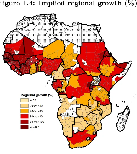
The geographic variation in growth due to IM A[ is shown in Figure 1.4 (using the estimates from column 1 of Table 1.6). The largest gains
are in West Africa, where in a number of regions growth in IM A[ alone implies a doubling of domestic output over the period. In the south, the regions bordering South Africa enjoy the highest levels of IMA, but have been adversely a¤ected by comparatively weak South African growth. This is particularly true for Botswana, southern Namibia and southern Mozam-bique, highlighting the importance of South Africa for the wider region’s
Figure 1.4: Implied regional growth (%)
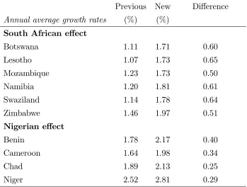
1.6.2 Case studies: South Africa and Nigeria
In this sub-section I quantify the importance of South Africa to the wider
Southern region, as well as Nigeria’s importance to West Africa. The two countries dominate the Sub-Saharan economy, together accounting for over half of total output and almost a quarter of intra-African imports in 2012.39
Here I demonstrate how their fortunes a¤ect their immediate neighbours, by calculating the change in each of their neighbours’growth rates resulting from a 1 percentage point annual increase in South African and Nigerian
growth.40
The results are presented in Table 1.7. The "previous" column shows the annual average growth rate in each country based on equation (16), as in Table 1.6 (using column (1),b = 0:665), and the "new" column repeats the calculation but with higher Yjt …gures for the South African and Nigerian
regions in IM A[it. For South Africa the largest gains accrue, as expected,
to Lesotho and Swaziland, where growth in each country expands by more than 0.6 percentage points per year. Mozambique gains the least of all the
neighbours, as South Africa is less important to the market access of its northern regions. Even here though, each addtional percentage point of growth in South Africa’s regions contributes an additional 0.5 percentage points of growth in Mozambique.
The impact of Nigerian growth is lower than that of South Africa owing both to its smaller economy and its higher trade costs with its neighbours.41
Its economic impact is still considerable however, with a 1 percentage point increase in growth re‡ected in at least a quarter of a percentage point of growth amongst each of its immediate neighbours.
41South Africa is a member of an RTA with all of its neighbours, and shares a currency
Table 1.7: E¤ect of higher South African & Nigerian growth Previous New Di¤erence Annual average growth rates (%) (%)
South African e¤ect
Botswana 1.11 1.71 0.60
Lesotho 1.07 1.73 0.65
Mozambique 1.23 1.73 0.50
Namibia 1.20 1.81 0.61
Swaziland 1.14 1.78 0.64
Zimbabwe 1.46 1.97 0.51
Nigerian e¤ect
Benin 1.78 2.17 0.40
Cameroon 1.64 1.98 0.34
Chad 1.89 2.13 0.25
Niger 2.52 2.81 0.29
Based on a 1% point annual increase in growth in each South African and Nigerian region.
1.6.3 Policy evaluation: West African currency union
It is argued above that Nigeria’s high trade costs reduce the extent to which its growth bene…ts its neighbours. More generally, any policy that lowers trade costs increases IMA and thus increases both growth spillovers and domestic output. Based on the gravity results, we can quantify the extent to which speci…c policies will increase IMA, and then based on the results in Table 1.4, we can estimate the impact of this policy on output.
In this sub-section I calibrate the impact of a speci…c policy with impli-cations for both Nigeria and the surrounding neighbourhood. Speci…cally, six West African countries - Gambia, Ghana, Guinea, Liberia, Nigeria and Sierra Leone - are proposing to enter into a CU, sharing a new currency called the eco.42 Ultimately, this CU will expand to incorporate the existing
http://www.economist.com/news/…nance-and-economics/21591246-continent-West African Economic and Monetary Union (WAEMU). As the primary motivation for a CU is to boost trade, in this section I calibrate the extent to
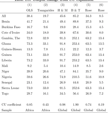
which this proposed CU would increase market access, and in turn increase output. I ask the following: how much higher would predicted output be in 2012 if the CU was in place?
The implied output change for each country is provided in Table 1.8. As the output change is very sensitive to how much a CU boosts trade, I consider a range of estimates from the literature. That is, in each column I
re-estimateIM A[ (in both the actual and counterfactual worlds), replacing the CU coe¢ cient from Table 1.3 with previous estimates from the liter-ature. Column (1) uses my estimate from Table 1.3 (column 4), column (2) uses the estimate of Tsangarides et al. (2008) as this is also based on African trade ‡ows, and column (3) uses the median estimate from Head and Mayer’s (2015) gravity meta-analysis. Columns (4) to (6) are based
on papers that have explicitly addressed the potential endogeneity of CUs: Barro and Tenreyro (2007), estimated using instrumental variables; Rose (2001), estimated with pair …xed e¤ects; and Rose (2001) estimated using a matching technique.
My baseline estimate in column (1) is that the proposed CU would boost aggregate West African output by almost 40 percent, based on the
predicted increase in trade. The biggest winners are the countries that are not members of the current CU, the WAEMU, as their trade costs with the entire WAEMU block are lowered. Based on the CU e¤ect estimated by Barro and Tenreyro (2007), the output of such countries would more than double. Such dramatic output gains are driven by their estimate that a CU
increases trade by over 500 percent. At the other extreme, the estimates in column (6), based on Rose’s matching technique, imply that such countries would gain an output boost o