Measurement of velocity profiles in multiphase flow using a multi electrode electromagnetic flow meter

Measurement of velocity profiles in multiphase flow using a

multi-electrode electromagnetic flow meter

T. Leeungculsatien

n

, G.P. Lucas

School of Computing and Engineering, University of Huddersfield, Huddersfield HD1 3DH, UK

a r t i c l e

i n f o

Available online 23 October 2012

Keywords: Velocity profile

Multi-electrode electromagnetic flow meter

Multiphase flow

a b s t r a c t

This paper describes an electromagnetic flow meter for velocity profile measurement in single phase and multiphase flows with non-uniform axial velocity profiles. A Helmholtz coil is used to produce a near-uniform magnetic field orthogonal to both the flow direction and the plane of an electrode array mounted on the internal surface of a non-conducting pipe wall. Induced voltages acquired from the electrode array are related to the flow velocity distribution via variables known as ‘weight values’ which are calculated using finite element software. Matrix inversion is used to calculate the velocity distribution in the flow cross section from the induced voltages measured at the electrode array. This paper presents simulations and experimental results including, firstly the effects of the velocity profile on the electrical potential distribution, secondly the induced voltage distribution at the electrode pair locations, and thirdly the reconstructed velocity profile calculated using the weight values and the matrix inversion method mentioned above. The flow pipe cross-section is divided into a number of pixels and, in the simulations, the mean flow velocity in each of the pixels in single phase flow is calculated from the measured induced voltages. Reference velocity profiles that have been investigated in the simulations include a uniform velocity profile and a linear velocity profile. The results show good agreement between the reconstructed and reference velocity profiles. Experimental results are also presented for the reconstructed velocity profile of the continuous water phase in an inclined solids-in-water multiphase flow for which the axial solids-in-water velocity distribution is highly non-uniform. The results presented in this paper are most relevant to flows in which variations in the axial flow velocity occur principally in a single direction.

&2012 Elsevier Ltd. All rights reserved.

1. Introduction

Conventional electromagnetic flow meters (EMFMs) have pre-viously been used successfully in varieties of industries for measuring volumetric flow rates of conducting fluids in single phase pipe flows. At present, a conventional EMFM can measure the volumetric flow rate of a single phase flow with an error as

low as 70.05% of reading provided that the velocity profile is

axisymmetric. However highly non-uniform velocity profiles are often encountered, e.g. just downstream of partially open valves. The axial flow velocity just downstream of a gate valve varies principally in the direction of the valve stem, with the maximum velocities occurring behind the open part of the valve and the minimum velocities behind the closed part of the valve. In such non-uniform velocity profiles the accuracy of the conventional

EMFM can be seriously affected[1]but high accuracy volumetric

flow rate measurements could be achieved by measuring the axial velocity profile and using this to determine the mean flow velocity in the cross section. Large variations in the axial flow velocity can also occur in multiphase flows e.g. horizontal and upward inclined multiphase flows in which axial velocity varia-tions occur principally in the direction of gravity, with the minimum axial velocity at the lower side of the inclined pipe and the maximum velocity at the upper side of the inclined pipe. A specific example of a multiphase flow which is of great interest to the oil industry is upward inclined oil-in-water flow. Such flows are ‘water continuous’ and so the multiphase mixture is electrically conducting allowing the use of electromagnetic flow meters. However since the water velocity varies from a minimum at the lower side of the inclined pipe to a maximum at the upper side of the inclined pipe this causes erroneous readings from a conventional electromagnetic flow meter. Another flow of interest to the oil industry occurs during the drilling of inclined oil wells when rock cuttings flow co-currently with water based drilling mud. Mixture density variations in the flow cross section, caused by settling of the rock cuttings, can cause variations in the axial mud velocity from positive (upward) values at the upper side of Contents lists available atSciVerse ScienceDirect

journal homepage:www.elsevier.com/locate/flowmeasinst

Flow Measurement and Instrumentation

0955-5986/$ - see front matter&2012 Elsevier Ltd. All rights reserved. http://dx.doi.org/10.1016/j.flowmeasinst.2012.09.002

n

Corresponding author.

the inclined well to negative (downward) values at the lower side. In view of the above, the objective of this paper is to describe a new non-intrusive electromagnetic flow metering technique for (i) measuring the axial velocity profile of single phase flows of conducting fluids and (ii) measuring the axial velocity profile of the conducting continuous phase of multiphase mixtures (such as horizontal and inclined oil-in-water flows and solids-in-water flows) in which the conductivity of the dispersed phase is very much lower than the conductivity of the continuous phase. [Note

that in a previous paper[2]it has been shown that the relatively

minor variations of fluid conductivity, which occur in the cross section of such multiphase flows, have only a minimal effect on the operation of electromagnetic flow meters. This is particularly true if the volume fraction of the non-conducting dispersed phase is less than about 0.4].

An alternative approach to accurate volumetric flow rate measurement in highly non-uniform single phase flows has been

proposed by authors such as Horner[3] and Xu et al. [4] who

described multi-electrode electromagnetic flow meters which are relatively insensitive to the flow velocity profile. However, this type of flow meter does not provide information on the local axial velocity distribution in the flow cross section. This can be a major drawback, particularly in a steady multiphase flow where, for

example, the volumetric flow rateQcof a given phase can only be

found by integrating the product of the steady local velocityvc

and the steady local volume fraction

a

cof the phase in the flow

cross section as follows

Qc¼ Z

A

vc

a

cdA ð1Þ

where in Eq.(1)Arefers to cross sectional area. The approach of

Horner [3] would be of no benefit in determining the water

volumetric flow rate in a highly inclined oil-in-water flow such as

that described above—but in such a flow, the distribution of the

local water velocityvw could be determined using the

electro-magnetic flow metering method outlined in this paper and the

distribution of the local water volume fraction

a

w could be

obtained non-intrusively using electrical resistance tomography

(ERT) [5] enabling the water volumetric flow rate Qw to be

determined according to Eq. (1). Although previous work on

velocity profile measurement using multi-electrode

electromag-netic flow meters is reported in the literature (see for example[6]

for a brief review) much of this previous work is not specifically aimed at multiphase flow measurement which is a major thrust of the work described in this paper. Also much of this previous work involves only simulations rather than the use of a practical device such as that described later in this paper.

The essential theory of electromagnetic flow meters (EMFMs) states that charged particles, in a conducting material which moves in a magnetic field, experience a Lorentz force acting in a direction perpendicular to both the material’s motion and the

applied magnetic field. Williams[7]applied a uniform transverse

magnetic field perpendicular to the line joining the electrodes and the fluid motion and his experiments revealed that for a uniform velocity profile the flow rate is directly proportional to the voltage

measured between the two electrodes. Subsequently Shercliff[8]

showed that the local current densityjin the fluid is governed by

Ohm’s law in the form of

j¼

s

ðEþvBÞ ð2Þ

where

s

is the local fluid conductivity,vis the local fluid velocity,

andBis the local magnetic flux density. The expression (vB)

represents the local electric field induced by the fluid motion,

whereasEis the electric field due to charges distributed in and

around the fluid. For fluids where the conductivity variations are relatively minor (such as the single phase and the multiphase

flows under consideration in this paper) Shercliff [8] simplified

Eq. (2) to show that the local potential U in the flow can be

obtained by solving

r

2U¼

r

UðvBÞ ð3Þ

For a circular cross section flow channel bounded by a number

of electrodes, with a uniform magnetic field of flux density B

normal to the axial flow direction, it can shown with reference to

[8]that, in a steady flow, the potential differenceUjbetween the

jth_{pair of electrodes is given by an expression of the form}

Uj¼

2B

p

a

ZZ

v xð ,yÞW xð ,yÞjdxdy ð4Þ

where v(x,y) is the steady local axial flow velocity at the point

(x,y) in the flow cross section, W(x,y)j is the so-called ‘weight value’ relating the contribution ofv(x,y) toUjandais the internal

radius of the flow channel. Eq.(4)can be discretized as follows

by assuming that the flow cross section can be divided into ^I

elemental regions

Uj¼

2B

p

a

X^I

n¼1 ^

vnW^n,jA^n ð5Þ

wherev^n andA^n are respectively the local axial velocity in, and

the cross sectional area of, thenth elemental region._W^_{n,jis the} weight value describing the contribution of the axial velocity in thenth elemental region to thejth potential differenceUj. If the

axial flow velocity is now assumed to be constant in each ofN

large regions, Eq.(5)can be written as

Uj¼

2B

p

a

XN

i¼1 vi

X^Ii

n¼^Ii1þ1 ^

Wn,jA^n ð6Þ

whereviis the axial flow velocity in theith large region. In Eq.(6) when the subscriptnis in the range^_I

i1þ1rnr^Iiit refers to the

elemental regions lying within theith large region. [Note also that

there are^Ii^Ii1elemental regions within theith large region and

that, by definition,^I0¼0]. An ‘area weighted’ mean weight value

wij relating the contribution of the velocity vi in the ith large

region to thejth potential differenceUjis given by

wij¼ P^Ii

n¼^Ii1þ1

^ Wn,jA^n

Ai

ð7Þ

where Ai is the cross sectional area of the ith large region.

Combining Eqs.(6)and(7)gives

Uj¼

2B

p

a

XN

i¼1

viwijAi ð8Þ

It will be shown later in this paper that Eq.(8)can be inverted

to enable estimates of the local axial flow velocity viin each of

N large pixels to be determined from N potential difference

measurementsUjmade on the boundary of the flow. Furthermore,

although Eq. (8) was derived on the assumption that the axial

velocity in each large pixel is constant, it will be seen that when this inversion method is used to solve for the velocity in each large

pixel then the values ofviobtained give a good approximation to

the mean axial velocity in each of the large pixels, in situations where there is some axial velocity variation within each large pixel. InSection 2of this paper it is shown how the weight valueswij can be calculated, for a particular magnetic flow meter geometry,

using finite element techniques. In Section 3 values of Uj are

calculated for a number of different simulated velocity profiles in

the EMFM. InSection 4of the paper, a reconstruction technique is

outlined which enables the pixel velocitiesvito be determined from

the weight valueswijand the boundary voltage measurementsUj.

obtained from this practical EMFM device in a multiphase flow are presented.

2. Numerical modeling of the electromagnetic flowmeter

2.1. Electromagnetic flow meter geometry

In order to calculate the weight valueswijit is necessary to use

finite element techniques to solve Eq. (2) to determine the

potential distribution within the electromagnetic flow meter for a variety of different flow velocity profiles (seeSection 2.3). It was

decided to use the COMSOL[9] finite element solver to do this

because its software also enables prediction of the magnetic field produced by the electromagnetic flow meter’s Helmholtz coil. The specification of the EMFM was that it consisted of a PTFE (polytetrafluoroethylene) flow pipe mounted within a Helmholtz coil. The EMFM contained 16 equispaced electrodes located at the

planez¼0, which was also the plane containing the centers of the

2 coils forming the Helmholtz coil. The inner diameter of the flow pipe was 0.08 m, the outer diameter was 0.09 m and its axial length was 0.3 m. The inner and outer diameters of the two coils forming the Helmholtz coil were 0.2048 m and 0.2550 m

respec-tively (refer toFig. 1(a)). A cylindrical domain with a diameter of

0.32 m and a length of 0.32 m represented the boundary of the

computing domain (Fig. 1). The boundary condition for the

simulations was that the component of the magnetic field normal to the boundary of the computing domain was set to zero.

In order to calculate the relevant weight values (seeSection 1)

potential difference measurements must be acquired from elec-trode pairs at the internal boundary of the flow pipe (at the plane

z¼0), these electrodes being in contact with the flowing medium.

Sixteen electrodes were placed at angular intervals of 22.5

degrees on the flow pipe boundary (refer toFig. 2) the electrodes

being denoted e1, e2 etc, with electrode e5 at the top of the flow cross section and electrode e13 at the bottom of the flow cross

section (Fig. 2). For the simple flow meter geometry described in

this paper the flow cross section was divided into seven pixels. The geometry of these seven pixels was chosen such that the chords joining seven pairs of electrodes were located at the geometric centers (in the y direction) of the pixels (refer to

Fig. 2). The fluid pixels are categorized as pixel 1 at the top of the flow cross section to pixel 7 at the bottom of the flow cross section. This pixel arrangement was chosen because, as described in Section 1, variations in the axial velocity in many flows of interest tend to occur in a single direction. Thus, for measuring the velocity profile behind a partially open gate valve, the flow

meter would be orientated such that the line joining e13 to e5 would be parallel to the valve stem (i.e. the direction of the magnetic field would be parallel to the valve stem). For making measurements in horizontal or inclined oil-in-water flows the line joining e13 to e5 would be in the direction from the

upper-most side of the pipe to the lowerupper-most side. The pixel areasAiare

shown inTable 1. In the simulations described in this paper, for

each simulated flow condition investigated, potential difference measurements were made between the seven electrode pairs

shown inTable 1 (the jth potential difference measurement Uj

was made between thejth electrode pair shown inTable 1). At the

plane of the electrodes, where z¼0, the local magnetic flux

density B was always perpendicular to both the fluid flow

direction and to the chords joining the electrode pairs (i.e. it

was in the y direction shown in Figs. 1 and 2). The fluid

-0.1 Cylinder defining computing domain

0 0.1

-0.1 -0.1 0 0.1

0.1 0

-0.1 0 0.1

0.1 0

-0.1

Flow channel Helmholtz

[image:3.595.337.511.230.376.2]

coil

Fig. 1.Schematic diagram of the electromagnetic flow meter used in the simulation. (a) 3D view and (b) View onx–y plane.

B

e13

e2 e4

e3 e6

e7

e8

e11

e14 e15 Flow Pixel

e10

e9 e1

e16

e12 e5

1

2

3

5

6

7

4

[image:3.595.303.554.452.545.2]

Fig. 2.Schematic diagram of the flow pixels, the electrodes and the direction of the magnetic field.

Table 1

Electromagnetic flow meter geometries.

Area Ai(m2) Electrode pairUj

(a) Pixel areas (b) Electrode pair Pixel1 (i¼1) 1.738 e4

Pair 1 (j¼1) e4–e6 Pixel2 (i¼2) 6.267 e4

Pair 2 (j¼2) e3–e7 Pixel3 (i¼3) 1.077 e3

Pair 3 (j¼3) e2–e8 Pixel4 (i¼4) 1.264 e3 _{Pair 4 (j}

¼4) e1–e9

Pixel5 (i¼5) 1.077 e3 _{Pair 5 (j}

¼5) e16–e10 Pixel6 (i¼6) 6.267 e4

Pair 6 (j¼6) e15–e11 Pixel7 (i¼7) 1.738 e4

[image:3.595.104.481.569.729.2]

conductivity used in the simulations was1.5102_Sm1

, this

conductivity value being typical of the mains water in the Huddersfield region of Northern England where the experiments

described inSection 6were carried out. In addition the flow pipe

was assumed to be made of PTFE with conductivity of 1

1015_Sm1_{, and the Helmholtz coil material was assumed to}

be copper with a conductivity of 5.96107_Sm1_.

[Note that for a sixteen electrode system, such as that shown inFig. 2, up to fifteen independent potential difference measure-ments could be made. With reference to the techniques described in Sections 1 and 4 of this paper, this would allow the flow velocity to be determined in up to 15 pixels into which the flow cross section could be divided. The sizes and shapes of these 15 pixels could be selected as required (provided that the relevant weight functions relating the pixel velocities to the boundary potential difference measurements are calculated). If the variation of the axial velocity was unlikely to be in a single direction then

instead of using the pixel arrangement shown inFig. 2, the use of

pixels of approximately square shape would be more appropriate. Note also that although in the study described in this paper electrodes e13 and e5 are not used, they would be required if additional pixels were used as described above].

2.2. Simulated magnetic flux density distribution

In the present investigation a Helmholtz coil was used to produce a near uniform local magnetic flux density distribution

in the flow cross section. COMSOL finite element software [9]

enabled simulation of the distribution of the magnetic flux density

Bin the computing domain produced by this Helmholtz coil. The

Helmholtz coil consisted of two identical circular coils placed symmetrically on each side of the PTFE flow pipe as shown in

Fig. 1. The coils were simulated such that electrical current flowed through both coils in the same direction and each coil carried the same current density. In the simulations described in this section, the current density in each coil was set such that the mean

magnetic flux density in the ydirection (see Figs. 1 and 2) was

110.4 G (110.4104_{T) in the flow cross section at the plane of}

the electrodes (wherez¼0). This was similar to the value of the

mean magnetic flux density in the y direction required for the

practical electromagnetic flow meter described in Section 5. In

the simulations, for this mean value of the magnetic flux density, the minimum and maximum values of the magnetic flux density in

the ydirection in the flow cross section at the plane z¼0 were

109 G and 112 G respectively, showing that the magnetic field was very close to being uniform in the flow cross section.

2.3. Calculation of the weight values

To numerically simulate the weight valueswij, relating the mean

flow velocity vi in the ith pixel to the jth potential difference

measurement Uj between the jth pair of electrodes on the flow

boundary, the flow channel is divided into seven pixels as described above (refer toFig. 2). The fluid in the pixel for which weight values are to be calculated is given an axial flow velocity (in thezdirection) greater than zero whilst the remaining pixels all have zero fluid velocity. The COMSOL finite element solver is then used to

deter-mine the distribution of the electrical potentialUin the computing

domain, for the magnetic flux density distribution in the flow cross

section, at the planez¼0, as given inSection 2.2above. [Note that

for this finite element simulation of the electrical potential distribu-tion, the number of mesh elements in the flow cross section at the

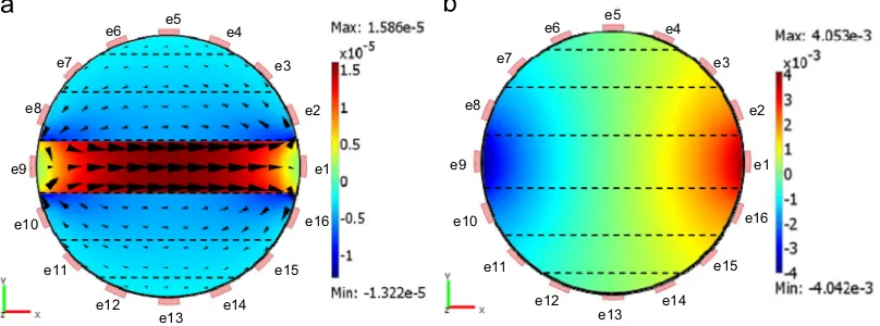
planez¼0 was 488].Fig. 3shows the distribution of the Lorentz

forces and the induced electrical potentials when the fluid in

pixel 4 has an imposed velocity in thezdirection while the fluid

in the remaining pixels is at rest. Fig. 3(a) illustrates the Lorentz force distribution arising from the imposed velocity in pixel 4. The magnetic field interacts with the charges carried in the water via these Lorentz forces causing the separation of charged ions (positive and negative) and giving rise to the electrical potential distribution shown inFig. 3(b). The arrows shown inFig. 3(a) also represent the direction of the local induced current density and it can be seen that for the (highly contrived) case in which flow occurs in pixel 4 only there is circulation of the electric current.

From the calculated potential distribution on the boundary of

the flow (see also Fig. 3(b)) the seven potential differences Uj

between the 7 electrode pairs given inTable 1can be calculated

allowing all of the weight valuesw4jassociated with pixel 4 to be

calculated according to Eq.(9)(withi¼4 andj¼1–7). The process

is then repeated for each of the other six pixels in succession until

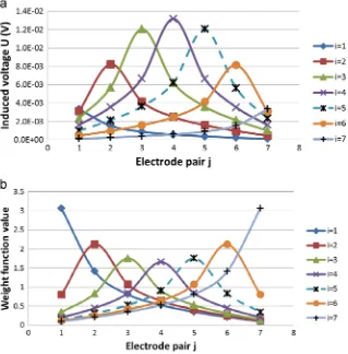
all relevant 49 weight values have been calculated.Fig. 4(a) shows

the induced voltages plotted against electrode pairs for all of the

seven simulations.Fig. 4(b) shows the 49 weight values calculated

from the induced voltages given inFig. 4(a) by using Eq.(9).

wij¼Uj

p

a 2B

1 viAi

ð9Þ

Note that the values ofwijcalculated according to Eq.(9)are

independent of the value ofviused in the simulation because, for

given values ofiandj,Ujis proportional tovi. The weight valueswij

calculated using Eq. (9) are equivalent to the values of wij that

would be obtained using Eq.(7). [NB: For a more detailed account of

the application of the weight value technique to electromagnetic flow metering the interested reader is referred to the seminal work

e1 e2 e4

e3 e6

e7

e8

e11

e12 e14

e15 e16

e13 e9

e10

e5

e1 e2 e4

e3 e6

e7

e8

e11

e12 e14 e15

e16

e13 e9

e10

[image:4.595.101.505.571.721.2]

e5

Fig. 3.(a) Simulation of Lorentz force distribution per unit volume [N/m3

of Shercliff [8]]. It is worth noting, with reference to[8], that if ‘point’ electrodes are assumed, then the local weight valueW(x,y)j (see Section 1) at the precise position of a point electrode can

sometimes be analytically calculated to be infinite. Eqs. (4)–(7)

indicate that an infinite local value ofW(x,y)jshould cause some of

thewijvalues to be infinite. Since the mesh elements used in the

simulations were of finite size it is unlikely that infinite values ofwij would have been observed, nevertheless the facts that (i) not even

exceptionally large values ofwijwere observed in the simulations;

and (ii) the calculated values ofwijenabled accurate velocity profile

reconstruction to be performed (seeSections 4 and 6), suggest that

infinite weight valuesW(x,y)jthat can be obtained analytically are

of little practical significance—almost certainly because they act

over an infinitesimally small region of the flow.

3. Effect of velocity profile on electrical potential distribution

The next stages of the investigation were; (i) to apply different simulated velocity profiles to a flowing single phase fluid (water);

(ii) to find the resultant induced potential differencesUj using

COMSOL; (iii) to reconstruct the single phase velocity profiles (see

Section 4); and (iv) to compare the reconstructed velocity profiles with the applied simulated velocity profiles. Two different simu-lated velocity profiles were investigated, a uniform velocity distribution and a linear velocity distribution as described below.

3.1. Uniform velocity profile

Fig. 5shows the potential distribution arising from an imposed

uniform, single phase (water), velocity distribution of 2 ms1_in

the flow cross section. The authors acknowledge that this velocity profile is unrealistic because fully developed, turbulent, single phase flows in circular pipes are generally axisymmetric with ‘1/7th power law’ velocity profiles. Nevertheless, as a means of investigating flow velocity image reconstruction techniques this uniform velocity profile is very useful in its simplicity.

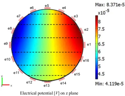
3.2. Linear velocity profile

[image:5.595.134.453.59.383.2]

Fig. 6shows the potential distribution arising from an imposed, linear single phase (water) velocity distribution in the flow cross section. The axial flow velocityvzin thezdirection is given by the Fig. 4.(a) Simulation results for the induced voltage between the j’th electrode pair when flow occurs only in the i’th pixel; and (b) resultant weight values relating the voltage between the j’th electrode pair to the velocity in the i’th pixel.

e1 e2 e4

e3 e6

e7

e8

e11

e12 e14

e15 e16

e13 e9

e10

e5

[image:5.595.316.540.425.576.2]

Electrical potential [V] on z plane

expression

vz¼1þ

y

a ð10Þ

whereyis the coordinate in the simulation in the direction shown in

Fig. 6 andais the internal pipe radius. This results in vz varying

linearly from zero aty¼ 0.04 m to 2 ms1

aty¼0.04 m. This type of linearly varying velocity profile has previously been reported in

[10](albeit for multiphase rather than single phase flows).

The relevant induced voltages Uj for the uniform velocity

profile and linear velocity profile were calculated for the electrode

pairs shown in Table 1. It should be noted that the electrical

potential distribution for the uniform velocity profile and linear velocity profile are entirely different from each other. For the uniform velocity distribution the induced voltages between pairs 1, 2 and 3 are the same as for pairs 7, 6, and 5 are respectively. For the linear velocity profile the induced voltage between pair 1 is higher than that for pair 7. Similarly the induced voltages between pairs 2 and 3 are respectively higher than for pairs 6 and 5. Moreover for the linear velocity profile the highest induced voltage is between electrode pair 3 while the maximum induced voltage for the uniform velocity profile is between electrode pair 4. Similar relationships between the velocity profile and the induced voltage distribution have also been previously observed[2].

4. Simulated velocity profile reconstruction

As mentioned earlier, the weight values wij are used to

reconstruct the mean velocityviin each pixel using the calculated

induced voltagesUj. The reconstruction method can be expressed

simply by the following matrix equation

V¼

p

a

2B½WA

1_{U ð11Þ}

In which V is a single column matrix containing the pixel

velocitiesvi,Wis a square matrix containing the relevant weight

values wij,Ais a diagonal matrix containing information on the

pixel areas Ai and U is a single column matrix containing the

calculated potential differences Uj for a given imposed velocity

profile. The inversion of [WA] was performed using a Tikhonov

regularization technique involving singular value decomposition (SVD) of [WA] (see for example[6]).

For the two velocity profile simulations that were undertaken

the reconstructed velocity profiles are shown inFig. 7(a) and (b).

Also shown in Fig. 7(a) and (b) are the original imposed velocity

profiles (which show the mean imposed flow velocity in each pixel)

from which the potential difference measurements Uj were

obtained. With close inspection of Fig. 7 it can be seen that the

reconstructed velocity profiles have reasonable agreement with the original imposed velocity profiles for both the uniform and linear velocity profiles.Fig. 7(a) shows that for the imposed uniform, single phase (water) velocity profile the maximum (most overestimated) and minimum (most under estimated) reconstruction errors occur

in pixel 1 (þ3.23%) and pixel 5 (2.31%) respectively. The most

accurate reconstructed velocity is in pixel 6 with an error of only 0.5%. The linear, single phase (water) velocity profile has maximum and minimum reconstruction errors in pixels 1 and 7 respectively. The most accurate reconstructed velocities for the linear velocity

profile are in pixels 3 and 6 with errors of 0.99%and 0.24%

respectively. The errors in the reconstructed linear velocity profile

may be due to violation of the assumption in Eq.(6)that the flow

velocity is constant in a given pixel. Nevertheless, despite this violation, the imposed linear profile can be seen to be reconstructed with reasonably good accuracy.

[Note that, as stated in Section 2.1, for a 16 electrode system

(such as that used in the present study) it is possible to make 15

independent potential difference measurementsUj, and so it would

actually be possible to divide the flow cross section into 15 rather than 7 pixels. It might be thought that a 15 pixel system would enable a more accurate reconstructed velocity profile to be obtained. However the accuracy of the velocity reconstruction method is

highly dependent upon the condition number of the matrix [WA]

e1 e2 e4

e3 e6

e7

e8

e11

e12 _e14

e15 e16

e13 e9

e10

e5

[image:6.595.63.272.363.524.2]

Electrical potential [V] on z plane

Fig. 6.Simulated induced potential distribution for the axial flow velocity varying linearly from 0 ms1

aty¼ 0.04 m to 2 ms1

[image:6.595.139.464.567.729.2]

aty¼ þ0.04 m.

and this condition number rises rapidly as the number of pixels is increased, making the technique more susceptible to measurement errors inUj. For the 7 pixel arrangement shown inFig. 2the condition

number of [WA] is 8.4, but for a typical 15 pixel arrangement the

condition number rises to about 130,000. Fig. 2 represents an

optimum arrangement, giving the maximum number of pixels for

which the condition number of [WA] is acceptably small].

The total volumetric flow rate Qw of the water can be

calculated from a reconstructed velocity profile as follows;

Qw¼

X7

i¼1

Aivi ð12Þ

whereAiis the area of theith pixel, andviis the reconstructed

velocity in the ith pixel. Let the true volumetric flow rate

associated with the imposed uniform velocity profile be Qwiu

and the volumetric flow rate associated with the reconstructed

uniform velocity profile beQwru. Also let the true volumetric flow

rate associated with the imposed linear velocity profile be Qwil

and the volumetric flow rate associated with the reconstructed linear velocity profile beQwrl. For the uniform velocity profileQwiu

is calculated to be 36.13 m3_hr1 _{and Q}

wru is found to be

35.71 m3_hr1_{. There is thus an error of only}

1.17% in the total

volumetric flow rate obtained from the reconstructed uniform velocity profile. For the linear velocity profileQwilis calculated to

be 18.06 m3hr1

, andQwrlis calculated to be 17.9 m3hr1. There

is thus an error of only 0.88% in the total volumetric flow rate

obtained from the reconstructed linear velocity profile.

5. A practical electromagnetic flowmetering device

A real imaging electromagnetic flow meter (see Fig. 8) was

constructed using the same geometry modeled in the COMSOL

simulations described above. The non-conducting flow meter body, with an internal radius of 80 mm, was made from Delrin. Four grooves on the flow meter body were machined to accom-modate two circular coils which formed a Helmholtz coil, with the mean spacing between the two coils being equal to the mean coil radius. The electrode array contained 16 electrodes for measuring flow induced potential differences, with each electrode being made from stainless steel. Stainless steel was chosen because (i) it has high corrosion resistance and (ii) it has a low relative permeability which meant that the electrodes did not significantly affect the magnetic field in the flow cross section.

Supports (labeled ‘E’ inFig. 8) were used to position the cables

running between the electrodes and the detection circuitry in such a way that they were always parallel to the local magnetic field. This meant that any ‘cable loops’ were not cut by the time

varying magnetic field—thus preventing non-flow-related

poten-tials from being induced in the cables.

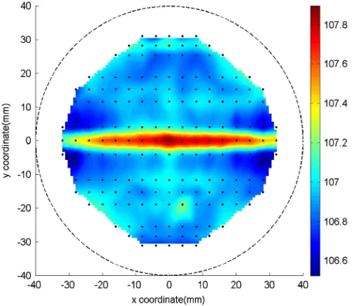
The technique described in this paper for measuring pixel flow velocities relies upon the magnetic flux density being uniform in theydirection (seeFig. 1) in the flow cross section at the plane of the electrodes. To check the uniformity of the magnetic field produced by the Helmholtz coil a 48 V dc power supply was connected to the two coils which were configured in parallel so that an equal current of 1.372 A flowed in the same direction in each coil. A ‘Hirst GM08 G-meter’ was then used to measure the

magnetic flux density in theydirection at 179 points in the flow

cross section at the plane of the electrodes. The results, which are

presented graphically inFig. 9, were analyzed to show that the

mean measured magnetic flux density in the flow cross section was 107.33 G, whilst the maximum and minimum measured values of the magnetic flux density were 107.89 G and 106.52 G, indicating the very near uniformity of the magnetic field strength. In normal operation, all measurement and control operations associated with the EMFM were made using a microcontroller.

Furthermore, the flow induced voltage between thejth electrode

pair was measured using the circuit shown in Fig. 10 which

consisted of two voltage followers and a differential instrumenta-tion amplifier with a gain of 996. A high pass filter was placed after each voltage follower to remove unwanted dc signals. A low

A: Meter Body

E: Cable Support

B: Helmholtz Coil

D: Electrode Array C: Flanges

A

E D

C

[image:7.595.64.253.418.727.2]

B

Fig. 8.Design of the electromagnetic flow meter used in the present study.

[image:7.595.303.554.478.696.2]

pass filter was placed after the differential amplifier to remove high frequency noise. In the present study, seven such circuits were required, one for each electrode pair.

A ‘hybrid square wave’ magnetic field was generated by switching the voltage supplied to the coils, from the 48 V dc power supply unit, using control signals supplied to a solid-state relay network. At any instant in time, the electrical current in

both coils had the same magnitude and direction.Fig. 11a is a

schematic of the variation of the mean magnetic flux densityBin

the flow cross section with time for this ‘hybrid square wave’, the purpose of which was to periodically reverse the direction of the flow induced potential at each electrode, thereby minimizing electrochemical effects at the electrode-water interface. The typical length of each cycle of the ‘hybrid square wave’ magnetic field used in the present investigation was 0.25 s and the

max-imum þBmax and minimum Bmax values of the mean

magnetic flux density in the flow cross section (in theydirection)

wereþ107.33 G and 107.33 G respectively. The transient time

t

c in the magnetic field, visible in Fig. 11a, was caused by a

transient in the current in each coil (when the coil voltage was switched) due to the coil inductance.

Each cycle of the hybrid square wave magnetic field can be

divided into four segments, denoted S1–S4 in Fig. 11a. Fig. 11b

shows one cycle of the jth flow induced voltage signal

Ux,jbetween thejth pair of electrodes in the electrode array. For

a given magnetic field cycle, mean values Ux,j

S1, Ux,j

S2,Ux,j

S3, andUx,j_S4were obtained from measurements ofUx,jfor each of the four signal segments S1to S4. Note that Ux,j

S1, Ux,j

S2,Ux,j

S3 and Ux,j

S4were obtained from measurements ofUx,jmade after

the relevant transient (of length

t

cfor S1and S3) was complete.

For a given magnetic field cycle, the relevant flow induced

potential differenceUjrequired for the pixel velocity calculation

(Section 4and Eq. (11)) was obtained from the average of the

difference between the jth measured voltages when B¼ þBmax

andB¼0 and the difference between thejth measured voltages

whenB¼0 andB¼ Bmaxas shown in Eq.(13)below. Division by

996 is required in Eq.(13)to compensate for the amplification of

the differential instrumentation amplifier described above.

Uj¼

9_Ux,j

s1Ux,j

s29þ9Ux,j

s3Ux,j

s49

2

1 996

ð13Þ

6. Experimental results in multiphase flow

Measurements of the local water velocity profile in a solids-in-water flow were made using the EMFM device described in

Section 5. The experiments were performed in the 3 m long 80 mm internal diameter working section of a multiphase flow

loop at the University of Huddersfield (see [10] for a more

complete description of the flow loop). For the experiments described in this paper the working section was either vertical (

y

¼01) or inclined at an angle of 301(

y

¼301) away from vertical. Electrically non-conducting spherical, plastic beads with an

aver-age diameter of 4 mm and a density of 1340.8 kgm3 _were

homogenously mixed with water in a holding tank before being pumped to the base of the working section. The flow rate of the multiphase mixture was controlled by varying the speed of a multiphase pump located between the holding tank and the

working section. The EMFM device described in Section 5 was

installed 2 m away from the inlet of the working section. At each

flow condition, voltages Ux,j (j¼1 to 7) (see Fig. 10) were

measured for the relevant electrode pairs over a period of 60 s

(with reference toSection 5, this meant that values of Ux,j

S1, Ux,j

S2,Ux,j

S3 and Ux,j

S4 were obtained from averaging data

from 240 magnetic field cycles, since each magnetic field cycle th

j electrode pair

U x,j

[image:8.595.49.288.244.337.2]

LP filter

Fig. 10.Electronic circuitry for measuring the flow induced potential difference between each electrode pair.

Bmax

+

( )

Ux,jS1

0 S1 S2 S3 S4

Time

Time

S1 S2 S3 S4

c c

B

j x U,

( )

Ux,jS3

Bmax

−

[image:8.595.49.288.382.553.2]

τ _τ

Fig. 11.(a) (top) Hybrid square wave magnetic field cycle. (b) (bottom) resultant flow induced potential difference forjth electrode pair.

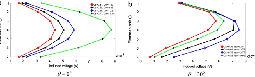
[image:8.595.85.523.598.730.2]

has a period of 0.25 s). Results for several multiphase flow

conditions are presented inFigs. 12 and 13. In these figures, for

y

¼01, the solids volumetric flow rate Q_s was in the range

0.51 m3_hr1_{to 0.98 m}3_hr1_{and the water volumetric flow rate}

Qwwas in the range 7.89 m3hr1to 15.74 m3hr1. For

y

¼301,Q_s

was in the range 0.36 m3_hr1_{to 0.75 m}3_hr1_andQ

wwas in the

range 8.34 m3_hr1_{to 13.77 m}3_hr1_{. These values ofQ}

sandQw are typical of those encountered in industrial slurry monitoring application in 80 mm diameter pipes.

For each flow condition investigated, the induced voltagesUj

(j¼1 to 7) were calculated from the measured values of Ux,j

S1, Ux,j

S2, Ux,j

S3 and Ux,j

S4 according to Eq. (13)and the

corre-sponding pixel velocitiesvi(i¼1 to 7) were then calculated from

these values ofUjaccording to Eq.(11). The values ofwijused in

calculating these pixel velocities were those presented inFig. 4b.

Fig. 12shows a plot of the values of Ujfor each electrode pair (refer toTable 1) for all of the flow conditions investigated.Fig. 13

shows a plot of the reconstructed pixel velocities for all of the flow conditions investigated.

The reconstructed velocity profiles illustrated inFig. 13(b) clearly indicate evidence of negative axial water velocity at the lower side of the inclined pipe, showing that in the seventh pixel, the water was flowing back down the pipe. Towards the upper side of the inclined pipe, the mean axial water velocity was large and positive indicating that the water was flowing quickly upward. These results agree well with visual observation of the flow undertaken using high speed

filming. Previous research (e.g.[10]) has reported similar phenomena

in inclined solids-in-water flows from results obtained using an intrusive six electrode local conductance velocity measurement

probe. Fig. 13(a) shows that for vertical solids-in-water flows the

water velocity is much more uniform in the flow cross section. Note

that the relatively uniform velocity profiles shown inFig. 13(a) are

typical of the velocity profiles that are seen over a much wider range of vertical solids-in-water flow conditions. Note also that the velocity

profiles shown inFig. 13(b) cover the extremes of velocity profile

shape encountered in many inclined (and other stratified) solids in water flows namely (i) relatively minor variations in velocity from pixel 7 to pixel 1, forQs¼0.75 m3hr1andQw¼13.77 m3hr1to (ii) marked backflow in pixel 7 to strong up-flow in pixel 1, for

Qs¼0.36 m3hr1andQw¼8.34 m3hr1.

With reference to Eq.(1), if the local solids and water volume

fraction distributions were known (for example by using

Elec-trical Resistance Tomography (see[5]and[10])) then an estimate

Qw,estof the water volumetric flow rate could be given by

Qw,est¼

X7

i¼1

vi

a

w,iAi ð14Þ

where

a

w,iis the mean water volume fraction in theith pixel and

Aiis the cross sectional area of theith pixel. If the simplifying

assumption is made that there is only very small local slip

between the phases an estimate Qs,est of the solids volumetric

flow rate could be given by

Qs,est¼

X7

i¼1

vi

a

s,iAi ð15Þ

where

a

s,iis the mean solids volume fraction in theithpixel.

7. Conclusions

This paper describes a measurement technique for mapping velocity profiles in single phase and multiphase flows. The results described in this paper are mainly relevant to flows in which the

axial flow velocity variesprincipallyin a single direction such as

(i) flows behind partially open valves or (ii) horizontal and inclined multiphase flows in which the continuous phase is electrically conducting. However by using alternative pixel arrangements the technique could be adapted to flows in which the axial velocity profile variation is not principally in a single direction. A weight value theory for an electromagnetic flow meter with multiple electrodes has been implemented and proved to be a valid method for relating the mean flow velocity in a pixel to the potential differences measured between various pairs of electrodes. More-over, this paper has used a matrix inversion method that can be combined with the weight values to reconstruct the mean velocity in each of a number of pixels from a given set of boundary potential difference measurements. In simulations, reconstructed velocities give good agreement with the reference pixel velocities and the reconstructed velocity profiles enable reasonably accurate volumetric flow estimates to be made. Experimental results for the measured water velocity profile, obtained in upward solids-in-water flows inclined at 01and 301to the vertical using a real multi-electrode electromagnetic flow meter, agreed well with the observed water velocity profile obtained from high speed filming. It is believed that the application of the techniques described in this paper to the measurement of highly non-uniform velocity profiles in multiphase flows is novel.

References

[1] Won Lim K, Chung MKyoon. Numerical investigation on the installation effects of electromagnetic flowmeter downstream of a 901elbow–laminar

flow case. Flow Measurement and Instrumentation 1999;10(3):167–74. [2] Wang JZ, Tian GY, Lucas GP. Relationship between velocity profile and

distribution of induced potential for an electromagnetic flow meter. Flow Measurement and Instrumentation 2007;18(2):99–105.

[3] Horner B. A novel profile-insensitive multi-electrode induction flowmeter suitable for industrial use. Measurement 1998;24(3):131–7.

[image:9.595.80.515.58.199.2]

[4] Xu LJ, Li XM, Dong F, Wang Y, Xu LA. Optimum estimation of the mean flow velocity for the multi-electrode inductance flowmeter. Measurement Science and Technology 2001;12:1139–46.

[5] Wang Mi, Ma Yixin, Holliday N, Dai Yunfeng, Williams RA, Lucas G. A high-performance EIT system. IEEE Sensors Journal 2005;5(2):289–99.

[6] Lijun Xu Ya, Wang, Dong Feng. On-line monitoring of nonaxisymmetric flow profile with a multielectrode inductance flowmeter. Instrumentation and Measurement, IEEE Transactions on 2004;53(4):1321–6.

[7] Williams EJ. The induction of electromotive forces in a moving liquid by a magnetic field, and its application to an investigation of the flow of liquids. Proceedings of the Physical Society 1930;42:466–78.

[8] Shercliff JA. the Theory of Electromagnetic Flow-Measurement. New Ed. Cambridge University Press; 1987.

[9] COMSOL Corporation Femlab 3.5a User Guide; 2005.