Essays in Applied Economics
London, September 2019
Giulia Bovini
Declaration
I certify that the thesis I have presented for examination for the PhD degree of the London School of Economics and Political Science is solely my own work other than where I have clearly indicated that it is the work of others (in which case the extent of any work carried out jointly by me and any other person is clearly identified in it).
The copyright of this thesis rests with the author. Quotation from it is permitted, provided that full acknowledgement is made. This thesis may not be reproduced without my prior written consent. I warrant that this authorisation does not, to the best of my belief, infringe the rights of any third party.
I declare that my thesis consists of approximately 75,000 words.
Statement of conjoint work
I confirm that Chapter 1 was jointly co-authored with Matteo Paradisi and I con-tributed 50% of this work.
I confirm that Chapter 3 was jointly co-authored with Andr´es Barrios Fern´andez and I contributed 50% of this work.
Statement of use of third party for editorial help
I would like to express my profound gratitude to my supervisor Steve Pischke, for the excellent supervision, caring guidance and continued support throughout the PhD journey. I have benefitted from fruitful interactions with the faculty of the LSE Economics Department, in particular with the members of the CEP, the Labour Economics group, the Public Economics group and the Economics of Education group. I thank them all.
I gratefully acknowledge financial support from the UniCredit Foundation and I am thankful to Annalisa Aleati and Giannantonio De Roni for their encouragement. I am also grateful for the generous financial support provided by the LSE Economics Department.
Parts of the analyses presented in this dissertation have been carried out at the Italian Social Security Institute (INPS), thanks to the VisitINPS Initiative. I am thankful to all those who have been involved in setting up, sponsoring and man-aging the visiting program. In particular, I thank Tito Boeri, Pietro Garibaldi, Massimo Antichi, Maria Domenica Carnevale, Maria Cozzolino, Edoardo Di Porto, and Paolo Naticchioni. I am also thankful to Massimo Ascione, Elio Bellucci, Luca Cammarata, Vito La Monica and Marcella Nunzi, as well as to all the staff of Di-rezione Centrale Studi e Ricerche.
I thank my co-authors Andr´es Barrios Fern´andez and Matteo Paradisi, for having shared their knowledge and intellectual curiosity with me.
I would like to thank Paolo Sestito, Matteo Bugamelli and Eliana Viviano at the Bank of Italy, for encouraging me to continue and finish this journey. I am also thankful for the support received from all my colleagues in the Households and Labour Market Division, as well as from many friends in other divisions. I declare that the views and opinions expressed in this dissertation are mine and do not nec-essarily reflect those of the Bank of Italy.
In London I met several new friends and I am glad to have shared this journey with them. I thank, among others, Alexia, Andr´es, Felix, Francesco, Gianpaolo, Giulia, Giuseppe, Inna, Marta, Matteo, Monica, Nicola, and Vincenzo.
Abstract
The first chapter examines how an increase in statutory retirement ages affects in the short-run firms’ labour demand for older workers on the cusp of retirement, their co-workers and outsiders. By leveraging administrative data and a pension reform that in 2011 suddenly and heterogeneously raised statutory retirement ages in Italy, the paper finds effects on firing and hiring that are consistent with substitutability among different types of workers. It also documents changes in the take-up of other social insurance programs. This caused leakages on the revenues raised on a firm’s employees by the reform.
The second chapter studies whether pension reforms affect labour supply before in-dividuals come close to the retirement and benefit claiming decisions. By relying on administrative data, the paper examines the labour supply dynamics of a sample of Italian private-sector workers who were aged 35-45 in 1995, when a pension reform changed the way of calculating their social security benefits. Workers are observed until they reach ages between 46 and 56: during this period, at most small adjust-ments to labour supply are documented. Heterogeneity analyses explore whether the extent of the adjustments differs across socio-demographic groups.
Declaration 1
Statement of conjoint work 1
Statement of use of third party for editorial help 1
Acknowledgments 2
Abstract 3
1 11
1.1 Introduction . . . 11
1.2 Related literature . . . 15
1.3 Institutional Setting . . . 17
1.3.1 The Italian pension system . . . 17
1.3.2 Statutory and observed retirement date . . . 18
1.3.3 The Fornero reform . . . 18
1.4 Data . . . 20
1.5 Empirical Strategy . . . 21
1.5.1 Treatment construction . . . 22
1.5.1.1 Individual shift in the full retirement date . . . 22
1.5.1.2 Firm-level shift in the full retirement date . . . 24
1.5.2 Empirical Specification and identifying assumptions . . . 25
1.5.2.1 Empirical specification . . . 25
1.5.2.2 Identification assumptions . . . 26
1.5.2.3 Placebo tests . . . 26
1.5.2.4 Balancing tests . . . 27
1.5.3 Descriptive Statistics . . . 27
1.6 Older workers delay retirement after the reform . . . 28
1.7 Labour demand responses to the reform . . . 29
1.7.1 Layoffs . . . 29
1.7.2 New Hires . . . 31
1.7.3 Do firms respond to retirement delays happening in the future? 31 1.7.4 Labour demand adjustments within and across occupation groups . . . 32
1.7.5 Heterogeneity by pre-reform turnover rates . . . 32
1.7.6 Sensitivity checks . . . 33
1.8 Discussion . . . 34
1.9 Workers’ earnings and take-up of other social insurance programs . . 35
1.9.1 Earnings of Incumbent Employees . . . 35
1.9.2 Pension benefits and spillovers to other social insurance pro-grams . . . 37
1.10 Implications of substitutability for the revenues raised on incumbents 38
1.10.1 An accounting model . . . 38
1.10.2 Empirical implementation and results . . . 40
1.10.3 Substitutability, spillovers and welfare in the short-run . . . . 41
1.11 Conclusions . . . 42
1.12 Figures . . . 43
1.13 Tables . . . 49
Appendices 55 1.A The Italian labour market . . . 55
1.B Additional details about the Fornero reform . . . 57
1.C Procedure to clean matched employer-employee data . . . 59
1.D Computation of years of qualifying contributions . . . 60
1.E Conceptual framework . . . 61
1.E.1 Labour demand model . . . 61
1.E.2 Alternative wage formation models . . . 63
1.E.2.1 Intrafirm bargaining over total surplus . . . 63
1.E.2.2 Intrafirm bargaining over profits . . . 64
1.E.2.3 Monopsonistic labour market . . . 65
1.F Matching procedure and the cost of layoffs . . . 66
1.G The Fiscal Externality . . . 67
1.G.1 Derivation of The Fiscal Externality . . . 67
1.G.2 Empirical implementation and results . . . 67
1.H Additional figures and tables . . . 69
2 96 2.1 Introduction . . . 96
2.2 Related literature . . . 99
2.3 Institutional setting . . . 101
2.3.1 The pre-1993 regime . . . 102
2.3.2 The 1992 Amato reform . . . 104
2.3.2.1 Provisions that affected all individuals in a similar way104 2.3.2.2 Provisions that affected workers differently due to grandfathering clauses . . . 104
2.3.3 The 1995 Dini reform . . . 105
2.3.4 How grandfathering clauses made similar workers different . . 107
2.4 Data . . . 111
2.5 Empirical strategy . . . 112
2.6 Results . . . 115
2.6.1 Main effects . . . 115
2.6.2 Robustness checks . . . 116
2.6.3 Heterogeneous effects . . . 117
2.7 Conclusions . . . 120
2.8 Figures . . . 122
2.9 Tables . . . 135
Appendices 145 2.A Additional details on the retirement benefit formulae . . . 145
2.B Simulation of the change of first year pension benefits . . . 147
2.C Computing years of SS contributions by the end of 1995 . . . 151
3 164
3.1 Introduction . . . 164
3.2 Related Literature . . . 167
3.3 Institutional Setting . . . 169
3.3.1 The Chilean School System . . . 169
3.3.2 The FSD Reform . . . 170
3.4 Empirical Strategy . . . 173
3.5 Data and sample . . . 176
3.6 Results . . . 179
3.6.1 Effect of the FSD on Achievement . . . 179
3.6.2 Heterogeneity by students’ backgrounds . . . 182
3.6.3 Heterogeneity by school type . . . 183
3.7 Conclusions . . . 186
3.8 Figures . . . 189
3.9 Tables . . . 193
Appendices 200 3.A Public and Charter Schools . . . 200
3.B Robustness Checks . . . 202
1.1 The distribution of the shift in the full retirement date . . . 43
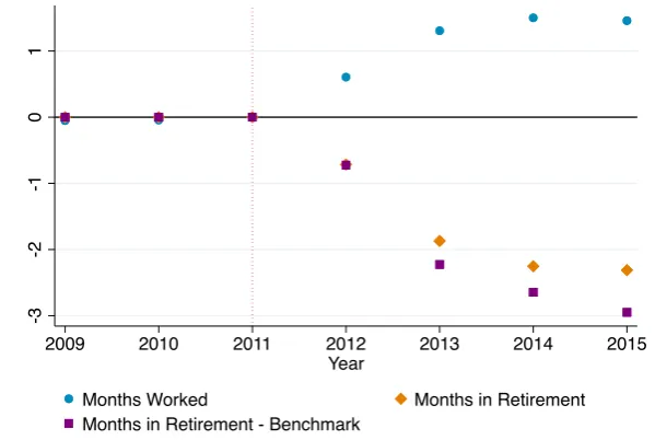
1.2 The effect of the reform on the working life ofpotential retirees . . . 44
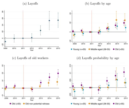
1.3 Labour demand adjustments: layoffs . . . 45
1.4 Labour demand adjustments: new hires . . . 46
1.5 Incumbents’ labour earnings . . . 47
1.6 Incumbents’ labour earnings, pension benefits and social insurance transfers . . . 48
1.H.1 Share of workers retiring at the full retirement date . . . 69
1.H.2 Age at retirement and number of new retirees by gender and type of pension . . . 70
1.H.3 Reform-induced changes in the full retirement date . . . 71
1.H.4 Post-reform retirement date - Forecast quality assessment . . . 72
1.H.5 Do firms respond to retirement delays happening in the future? . . . 73
1.H.6 Labour demand adjustments within and across occupation groups . . 74
1.H.7 Labour demand adjustments in firms with high and low turnover rates in the pre-reform period . . . 75
1.H.8 Labour demand adjustments: robustness to alternative specifications and samples . . . 76
1.H.9 Labour demand adjustments: layoffs by firm size . . . 77
1.H.10 Cost of Layoffs . . . 78
1.H.11 Co-workers’ earnings: the cost of layoffs vs within-firm dynamics . . 79
1.H.12 Co-workers’ earnings by age: the cost of layoffs vs within-firm dynamics 80 2.1 The 1992 Amato and the 1995Dini pension reforms . . . 122
2.2 Accrual rate in the Quota B and in the NDC regimes . . . 123
2.3 Yield rate in the Quota B and in the NDC regimes . . . 124
2.4 Distribution of years of Social Security contributions by 1995 for workers aged 35-45 and with 14 to 22 years of contributions . . . 125
2.5 Main results . . . 126
2.6 Main results, including observations very close to the threshold . . . 127
2.7 Placebo threshold at 19 years of SS contributions . . . 128
2.8 Placebo threshold at 20 years of SS contributions . . . 129
2.9 Main results, heterogeneity by gender . . . 130
2.10 Main results, heterogeneity by age in 1995 . . . 131
2.11 Main results, heterogeneity by (a proxy of) education . . . 132
2.12 Main results, heterogeneity by pre-1996 labour earnings . . . 133
2.13 Main results, heterogeneity by pre-1996 occupation . . . 134
3.1 FSD adoption over the period 1997-2013 . . . 189 3.2 Evolution of test scores relative to 1 year before the FSD adoption . 190
the FSD adoption . . . 191 3.4 Evolution of number of teachers, contract hours per teacher and
teaching hours per teacher relative to 1 year before the FSD adoption192 3.C.1 Evolution of the number of subjects relative to 1 year before the
1.1 Pre- and post-reform pension requirements . . . 49
1.2 Response of retirement choices to the change in the full retirement date . . . 50
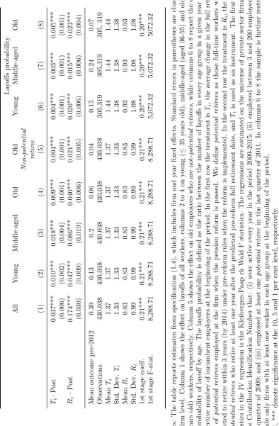
1.3 Labor demand adjustments: layoffs . . . 51
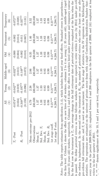
1.4 Labor demand adjustments: new hires . . . 52
1.5 Incumbents’ labour earnings . . . 53
1.6 Fiscal Externality . . . 54
1.H.1 Pre- and post-reform pension requirements - Additional Details . . . 81
1.H.2 Placebo tests . . . 82
1.H.3 Balancing tests . . . 83
1.H.4 Firms with at least onepotential retiree and other firms . . . 84
1.H.5 Potential retirees and other workers . . . 85
1.H.6 Potential retirees and other similar older workers: absences from work 86 1.H.7 The effect of the reform on the working lives of potential retirees . . 87
1.H.8 Labour demand adjustments: layoffs . . . 88
1.H.9 Labour demand adjustments: new hires . . . 89
1.H.10 Do firms respond to retirement delays happening in the future? . . . 90
1.H.11 Labour demand adjustments within and across occupation groups . . 91
1.H.12 Labour demand adjustments in firms with high and low turnover rates in the pre-reform period . . . 92
1.H.13 Incumbents’ labour earnings . . . 93
1.H.14 The effect of the reform on potential retirees and co-workers . . . 94
1.H.15 The components of the fiscal externality . . . 95
2.1 Sample summary statistics . . . 135
2.2 Main results . . . 136
2.3 Main results, including observations very close to the threshold . . . 137
2.4 Placebo thresholds at 19 and 20 years of SS contributions . . . 138
2.5 Main results, heterogeneity by gender . . . 139
2.6 Main results, heterogeneity by age in 1995 . . . 140
2.7 Main results, heterogeneity by (a proxy of) education . . . 141
2.8 Main results, heterogeneity by pre-1996 labour earnings . . . 142
2.9 Main results, heterogeneity by pre-1996 occupation . . . 143
2.10 Main results, heterogeneity along all dimensions together . . . 144
2.B.1 Simulation of the change in first year annual pension benefits stem-ming from post-1995 contributions . . . 150
2.E.1 Main results . . . 154
2.E.2 Main results, including observations very close to the threshold . . . 155
2.E.3 Placebo threshold at 19 years of SS contributions . . . 156
2.E.4 Placebo threshold at 20 years of SS contributions . . . 157
2.E.5 Main results, heterogeneity by gender . . . 158
2.E.7 Main results, heterogeneity by (a proxy of) education . . . 160
2.E.8 Main results, heterogeneity by pre-1996 labour earnings . . . 161
2.E.9 Main results, heterogeneity by pre-1996 occupation . . . 162
2.E.10 Main results, heterogeneity along all dimensions but age . . . 163
3.1 Daily schedules with and without the FSD . . . 193
3.2 Difference in hours of Instruction and voucher . . . 194
3.3 Use of time under the FSD . . . 195
3.4 Summary statistics . . . 196
3.5 Effect of the FSD on test scores . . . 197
3.6 Heterogeneous effects by students’ socio-economic Background . . . 198
3.7 Heterogeneous Effects by School Type . . . 199
3.B.1 Effect of the FSD on test scores including teacher controls . . . 204
3.B.2 Effect of the FSD on test scores - robustness checks . . . 205
3.C.1 Schools transfers and students’ characteristics . . . 209
3.C.2 Support received by students outside of school . . . 210
3.C.3 Frequency of mathematics homework . . . 211
3.C.4 Differences in autonomy by school type . . . 212
3.C.5 Evolution of teachers related inputs . . . 213
Labour substitutability and the impact of raising
the retirement age
1.1
Introduction
Substitutability among workers within the firm is crucial for the study of public policies. When a fraction of workers are targeted by a policy that alters incentives to work, spillovers on their co-workers may arise depending on whether the em-ployer finds close substitutes or complements among incumbent employees. Labour demand for outsiders can also be affected. These “hidden” micro-level effects have welfare implications that are hard to detect when looking at targeted individuals. Labour substitutability may exist along several worker’s characteristics: an example is substitutability between age cohorts that can affect the incidence of Social Secu-rity policies targeting older employees. In this paper, we propose a novel approach that regards firms as active agents in the analysis of delayed retirement policies and extends to other policies that lower the turnover of older workers.
Raising the retirement age provides older employees with incentives to postpone retirement.1 A rich literature documents the positive effects of these reforms on
old-age labour supply (e.g., Mastrobuoni, 2009; Staubli and Zweim¨uller, 2013).2 There
is, on the other hand, limited evidence on how firms adjust labour demand when older employees work for longer than expected. Do firms change their hiring and firing policies? Do labour demand adjustments affect earnings of incumbent employ-ees? Do these changes uniformly affect all cohorts of workers or disproportionately affect some of them? Answering these questions sheds light on the degree of sub-stitutability among workers of different ages within the firm. The extent to which
1Many governments have passed reforms that increase the retirement age to cope with
popu-lation aging and its threat to the sustainability of Social Security systems. The US is following such trends by committing to gradually adjust the full retirement age from 66 to 67 by 2022. The Congressional Budget Office has suggested further raising the statutory age to 70 to help reduce the budget deficit between 2017 and 2026 (Congressional Budget Office, 2016). Most European countries have implemented similar measures since 2000 (Carone et al., 2016).
2Other papers on how public pension systems affect retirement behaviour are Behaghel and
Blau (2012), Cribb et al. (2016), Lalive et al. (2017), Manoli and Weber (2018), Fetter and Lock-wood (2018) and Seibold (2019). This literature documents bunching in retirement at statutory retirement ages and large responses of retirement choices to statutory retirement ages.
has important implications for the effects of delayed retirement policies as well as of other policies that similarly reduce the turnover of older workers. Therefore, it is primarily important to assess firm responses to changes in the design of Social Security. In addition, since revenues raised on a firm’s employees by an increase in the statutory retirement age are a key component of welfare, it is crucial to examine whether and how they are affected by labour substitutability within the firm.
To address these questions we exploit the quasi-experimental variation of a unique pension reform implemented in Italy in 2011 - theFornero reform - that caused sud-den, substantial and heterogeneous changes in the full retirement age,i.e. the age at which workers can claim full pension benefits.3 We link matched employer-employee
records for small and medium firms to novel records that track all contributions to Social Security accumulated by their workers (more than 6 million individuals, over one third of private employees in 2009). Leveraging this novel match of different data sources, we can build firm-level measures of the reform-induced shock to the retirement date of older employees and we can study whether it affects firms’ firing and hiring decisions. Furthermore, we can observe the entire career of all workers and their take-up of various social insurance programs.
We start by investigating whether and how employers change their demand for labour in response to the reform. The results are informative about the degree of substitutability between workers within and across age cohorts. We then document how a higher full retirement age affects labour earnings and the take-up of social in-surance programs of older employees and - due to labour substitutability within the firm - of their co-workers. We conclude by discussing the implications of micro-level substitutability for the revenues collected by the reform from a firm’s employees in the short-run. To this end, we incorporate the demand-driven behavioural responses into the estimation of the fiscal externality of the policy, i.e. the leakages on the revenues that the government hopes to raise on a firm’s employees. We thus im-prove upon the existing literature that focuses on the behavioural responses of older workers. This exercise represents a first step to evaluating the importance of labour substitutability and firms’ decisions for the analysis of Social Security policies.
Estimating labour demand responses to reforms that increase the full retirement age poses two main identification challenges. First, most pension reforms are an-ticipated. Confounding anticipation effects make it hard to isolate firms responses. Second, the share of employees whose retirement date is delayed in the short-run, which is an intuitive metric of the reform shock, depends on the workforce age dis-tribution. Workers’ demographics vary across firms possibly due to differences in
3The full retirement age is intended throughout the paper as the age at which workers can
labour demand trends and other unobservable, time-varying characteristics. Hence, firms with a high concentration of younger workers, which are not affected much by the reform, may not serve as credible controls.
The features of the 2011 Italian pension reform allow us to address both identifica-tion issues. The reform was enacted by a newly appointed technocratic government in December 2011 and entered into effect in January 2012, leaving limited room for anticipatory effects. The new law raised the age and contribution requirements for old-age and seniority pensions. The design of the policy generated heterogeneous changes in the years until retirement eligibility across otherwise similar older work-ers. Specifically, these changes depend on gender and on small differences in the other two ingredients that determine eligibility, i.e. age and years of retirement contributions. As a result, firms with a similar workforce composition experienced differential shifts in the retirement date of employees who were expected to retire soon.
We leverage this feature of the reform to address the endogeneity problem. We restrict our attention to the subset of full-time workers on the cusp of retirement at the time of the reform. We then construct a treatment that measures the average firm-level shift in the full retirement date of these employees. The treatment is only weakly related to the demographics of the firm’s workforce in the data; this is be-cause it leverages small idiosyncratic differences across firms in the distribution of age, years of contributions and gender within the narrow subset of employees on the cusp of retirement. Neither does the treatment predict differences in labour demand trends in the pre-reform period. Furthermore, it has a direct economic interpreta-tion as a firm-level shift in the policy parameter, i.e. the retirement date of older workers. For this reason, in the second part of the paper we use it to study the short-run effect of raising the full retirement age on the revenues collected from a firm’s employees. In the first part of the paper, to document substitutability be-tween workers, we also use the treatment as an instrument to estimate how many individuals are fired or hired when an additional senior employee delays retirement.
also fired, causing spillovers within the firm. In particular, the percentage increase in firing is higher for older co-workers than for younger ones, indicating a closer substitutability with older workers expected to retire soon. Delaying the retirement date of an additional older worker also reduces hirings by 0.35 units (7 per cent of the pre-reform average). The decline is largely explained by fewer young and middle-aged new hires under temporary contracts. The effect on dismissals and hiring is concentrated within incumbent workers or outsiders who share the same qualifications (blue-collar, white-collar or manager) as older employees on the cusp of retirement.
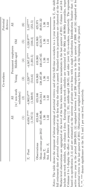
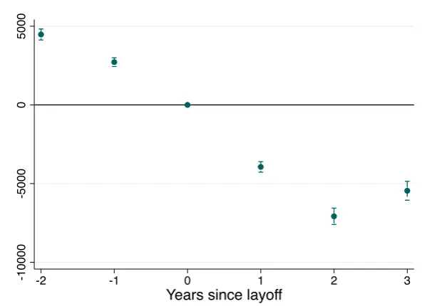
In the second part of the paper, we study how the reform affected workers on the cusp of retirement and - due to labour substitutability within the firm - their co-workers. We look at labour earnings and the take-up of social insurance programs. We associate each employee to the firm where he/she worked at the reform date. Then, we aggregate the outcomes of interest across workers of the same type (on the cusp of retirement or co-workers) who were incumbent at the same employer. We find that the pension reform has a positive effect on the earnings of employees close to retirement as they work for longer, but a negative effect on co-workers’ earnings. A 1-year shift in the full retirement date of workers close to retirement leads to a 11,356 euros drop in total labour earnings of co-workers in 2015, equivalent to 1.8 per cent of their average value in the pre-reform period. The decline in earnings becomes smaller when we take non-work subsidies into account. Hence, part of the observed dynamics reflects an increased layoff risk. We perform a calibration to infer what share of the drop can be attributed to layoffs. We find that firing explains around one-fifth of the earnings drop. The remaining part of the loss is likely attributable to within-firm earnings dynamics. The latter are more relevant for older and middle-aged employees, consistent with a model where the firm job ladder is based on seniority and the closer substitutes for senior employees on the cusp of retirement are older and middle-aged co-workers.
Stricter criteria for pension eligibility reduce the amount of pension benefits received by employees on the cusp of retirement, but increase - to a lower extent - their take-up of non-work subsidies and disability benefits. The receipt of non-work subsidies also increases among co-workers. Hence, a comprehensive evaluation of the short-run revenues raised by the reform needs to take into account the consequences on work-ers who are not directly affected by the policy and that arise due to the behaviour of firms. The previous literature has focused on the behavioural responses of older workers (e.g. Staubli and Zweim¨uller 2013; Vestad 2013). We show that spillovers on their co-workers - caused by labour substitutability - are also very important.
from a firm’s employees in the short-run, we develop an accounting model. Our framework allows for spillovers on co-workers and takes into account the effects of the reform on labour tax revenues and other social insurance programs. Using the model, we estimate the fiscal externality of the policy, i.e. the share of mechanical savings on the pension payments to a firm’s employees that the government loses be-cause of the behavioural responses of these employees and of the firm. According to our estimates, about two-thirds of the savings are lost in the short-run. The cost is entirely explained by spillovers on co-workers. By ignoring these spillovers, we would estimate a positive fiscal externality: higher labour tax revenues on older workers would more than offset costs stemming from their increased take-up of other social insurance programs. We therefore conclude that labour substitutability is pivotal to assessing the consequences of this reform and potentially similar policies that lower the turnover of older workers.
The remainder of the paper proceeds as follows: Section 1.2 reviews the related literature; Section 1.3 illustrates the institutional setting; Section 1.4 describes the data; Section 1.5 outlines the identification strategy; Section 1.6 shows that older workers delay retirement in response to the policy; Section 1.7 presents the main findings on firms’ labour demand adjustments; Section 1.8 discusses the main re-sults in relation to the literature; Section 1.9 documents the effect of the reform on co-workers’ earnings; Section 1.10 builds a model to estimate the revenues effects of the reform; Section 1.11 concludes.
1.2
Related literature
Our paper relates to the literature that explores the substitutability between workers within the firm using a firm’s responses to unforeseen shocks to its work-force. J¨ager and Heining (2019) exploit sudden workers’ deaths.4 While they
lever-age a negative shock to the retention rate, we study a positive one. Unlike a single worker’s death, a higher full retirement age may affect the retirement choice of more than one incumbent worker, providing a larger shock to a firm’s workforce. More-over, since our shock affects older employees, it allows us to study substitutabilities between workers within and across age cohorts. We relate our findings to labour de-mand theory and contribute to the understanding of labour substitutability within firms as studied in models with heterogeneous labour and imperfect labour markets (Cahuc et al., 2008 and Pissarides, 2000). We also add evidence on changes in in-ternal labour market dynamics (Baker et al., 1994).
Our study of the implications of labour substitutability for the revenues raised by
4Other recent papers that exploit sudden deaths or hospitalization events to study the
erosity of a given social insurance program affects the take-up of other programs.5
Closely related to our work is Staubli and Zweim¨uller (2013) who examine a reform increasing the early retirement age.6 Like them, we show that changes to Social
Se-curity rules can generate spillovers on other government programs. We bring a new perspective by treating the firm as an active agent for the transmission of the effects of a pension reform. To do so, we include in our accounting model the demand-driven spillovers on incumbent workers who are not directly affected by the policy in the short-term.
We provide firm-level evidence of substitutability within and across age cohorts. Several papers have studied the relationship between young and older employment within countries or sub-national macro-areas.7 Gruber and Wise (2010) conclude
that the correlation is positive looking at country case studies. More recent work by Bertoni and Brunello (2017) exploits variation in the age structure of Italian provinces and regions. They find that pension reforms causing fewer older workers to retire have negative effects on youth employment, especially during recessionary periods. Exploiting variation in the age structure of the older population across US commuting zones, Mohnen (2019) finds that the retirement slowdown is asso-ciated with increased unemployment and occupational downgrading among young individuals. As we discuss later, our results can be regarded as an evidence of the micro-level mechanisms that could deliver substitutability at a macro-level.
Recent and limited literature uses micro-data to investigate how pension reforms that affect elderly labour force participation change labour demand at the firm level. Vigtel (2018) shows that a decrease of the legal retirement age in Norway increases the hiring of senior workers, especially of “risky types” (blue-collar and with previ-ous records of sickness). Martins et al. (2009) study a Portuguese pension reform that increased the legal retirement age for women, finding negative effects on hiring, especially of younger female workers. Boeri et al. (2017) and Carta et al. (2019) evaluate the effects of the Fornero pension reform on employment. The former doc-ument a reduction of youth employment, whereas the latter find positive effects on young and middle-aged employment in a sample of large firms. Our new contribu-tion is threefold. First, we propose a novel identificacontribu-tion strategy that exploits firm idiosyncratic variation in treatment intensity unrelated to broad firm
demograph-5Some examples are works on the spillovers of changes in the disability insurance (Karlstr¨om
et al., 2008; Borghans et al., 2014; Staubli, 2011) or unemployment insurance (Lammers et al., 2013; Inderbitzin et al., 2016). Program substitution effects are also studied by Kline and Walters (2016).
6Vestad (2013) also studies how changes to early retirement provisions affect other social
insur-ance programs; Duggan et al. (2007) examine the spillovers on disability insurinsur-ance of a change in the full retirement age in the US; Atalay and Barrett (2015) explore how increasing the minimum age for women to claim the age pension in Australia affects the take-up of disability benefits.
7In a recent strand of literature, Acemoglu and Restrepo (2019) study the interaction of
ics. Second, we study separately layoffs of incumbent permanent workers and new hires of outsiders; this allows us to explore the susbstitutability among incumbent workers of different ages and the substitutability between incumbent workers close to retirement and individuals outside the firm. Third, we study the relevance of spillovers within the firm to provide novel evidence on the importance of firms for the incidence of these types of policies.
1.3
Institutional Setting
This section describes the main features of the Italian pension system. We provide statistics and institutional details on the Italian labour market in Appendix Section 1.A.
1.3.1 The Italian pension system
As for many OECD countries, including the US, the main pillar of the Ital-ian public pension system is a compulsory pay-as-you-go scheme.8 A combination
of earnings-related and contributions-related methods determines pension benefits. The Social Security tax rate on private payroll employment is 33 per cent. Statutory incidence falls on the employee for one-third and for the remaining two-thirds on the employer.
There are two options for claiming full retirement benefits: old-age pensions and seniority pensions. The eligibility criteria for both options have been substantially redesigned by the 2011 Fornero pension reform. The main early retirement op-tion, called opzione donna, is available for women only; it allows women to claim benefits before satisfying the old-age or seniority pension requirements. Similarly to early retirement in the US, until 2011 opzione donna allowed the claiming of benefits about 3 years before the statutory age.9 Exercising the early retirement
option comes at the cost of receiving lower pension benefits.10 The average cut is estimated to be roughly 35 per cent of the full benefits that an individual would be entitled to if choosing the seniority retirement option (INPS, 2016). Working past eligibility to retirement is allowed, although protection against dismissals is reduced
8In 2015 only 7.3 million people (less than one-third of people employed) had supplementary
private pension plans (COVIP, 2015). Although the number has been growing in recent years, the limited diffusion of these financial instruments is partly due to the fact that the public pension system is relatively generous.
9Early retirement usingopzione donna was possible in 2011 upon turning 57 years old (with 35
years of contributions). In the same year, private sector female employees could claim an old-age pension upon turning 60 years old (with 20 years of contributions).
10This is in part due to the fact that pension benefits are calculated using a fully
1.3.2 Statutory and observed retirement date
How retirement choices change in response to pension reforms that extend the full retirement date determines the extent to which firms experience an increase in the retention rate of older employees when these policies are implemented. We define an individual as retired when he/she starts collecting retirement benefits. Retirement spikes around the earliest among statutory full retirement dates in our data; more than 70 percent of individuals retired within a 1-year window around such a date in 2012 (Appendix Figure 1.H.1). This trend is common to other countries. In the US the share of workers retiring at the full retirement age has been increasing in the last decade; the share of individuals exercising the early retirement option has also starkly dropped (Munnell and Chen, 2015). Estimates in Mastrobuoni (2009) for the US document a strong response of retirement choices to the full retirement date: an increase in the full retirement age by 2 months increases the age at retirement by around half as much. A similar response emerges from our data where a one year shift in the full retirement date translates into a 7-month delay in retirement (see Section 1.6).
1.3.3 The Fornero reform
The Fornero pension reform was passed in December 2011 (Decree Law 201/11, article 24). It was part of the “Save Italy” decree, an emergency package of measures in response to the mounting pressure of financial markets on the Italian sovereign debt. Designed by a new technocratic government and approved one month after its appointment, it entered into force in January 2012. Although the need for a deficit reduction package was anticipated, its exact content was not known in advance. Moreover, the decision and implementation lags were both very short. As a result, anticipatory effects were likely negligible. The reform raised the requirements for claiming old-age and seniority pensions, reducing the number of new retirees and increasing the average age at retirement.12 The new dispositions applied to all
workers who did not accrue the right to claim retirement benefits under pre-reform rules by the end of 2011. A few other categories of workers - listed in Appendix Section 1.B - were grandfathered. For all other private sector employees, Table 1.1 compares the main features of pre- and post-reform retirement rules over the period
11In particular, the age and years of contributions are those needed by men for claiming an
old-age pension.
12Appendix Figures 1.H.2 plots the evolution of age at retirement and of the number of new
2012-2015, for old-age (Panel a) and seniority (Panel b) pensions. Appendix Table 1.H.1 and Appendix Section 1.B provide further details.
Old-age pensions: The reform raised the age requirement for old-age pensions,
whilst leaving the contribution requirement (20 years) unchanged. In 2011 the statutory retirement age was 60 for women and 65 for men. Absent the reform, it would have risen gradually to reach 61 years and 10 months for women and 65 years and 7 months for men in 2018. Per effect of the reform, the age requirement has further increased, to reach 66 years and 7 months for both genders in 2018. Hence, the change in the age requirement was considerably larger for women than for men.
Seniority pensions: The reform re-designed the rules for claiming seniority
pen-sions. Until 2011 a “quota” system was in place; workers could retire as soon as their age and years of contributions summed up to a “quota”, conditional on both surpassing a certain threshold. In 2011 the quota was set to 96, conditional on being at least 60 years old and having at least 35 years of contributions. Had the rules not changed, the “quota” would have gradually risen from 96 to 97.6 over the 2012-2108 period.13 Alternatively, workers could retire upon totalling 40 years of
contributions, regardless of their age. The Fornero reform abolished the “quota” system. It legislated that in 2012 a seniority pension could be claimed upon totalling at least 41 years and 1 month of contributions for women and 42 years and 1 month of contributions for men; the requirement gradually increased to reach 41 years and 10 months and 42 years and 10 months in 2018, respectively.14
The reform did not abolish the early retirement option. The take-up of such op-tion was very low until 2011, because of the cut in benefits. After the reform, which substantially tightened eligibility criteria for claiming full benefits, the take-up of opzione donna increased. Yet, even in the year when it peaked within our sample period (2015), less than 20 per cent of eligible women claimed early retire-ment. Moreover, only 80 per cent of them made job-to-retirement transitions (INPS, 2016).15 As a result, the take-up of opzione donna remains limited in our sample. The reform caused heterogeneous changes in years until retirement eligibility among otherwise similar older workers. As a result, firms with a similar senior workforce were affected by the reform to a different extent. Appendix Figure 1.H.3 shows the relationship between age and years of contributions in 2011 and the shift in the
13The age requirement for the “quota” 97.6 would have been 61 years and 7 months.
14If individuals start collecting retirement benefits before age 62, there is a 1 per cent penalty
for every year between the ages of 60 and 62, which raises to 2 per cent for every year before the age of 60.
benefits by 2014 under pre-reform rules. The heatmap highlights the substantial variation in the extent of the shift. Among female workers, the most affected are those between 58 and 59 years old with less than 35 years of contributions in 2011. Their retirement age shifts by 4 years or more.17 Women with more than 36 years of
contributions or who are closer to 60 years old experience smaller changes. Among male workers, those close to eligibility under “quota 96” are the most affected. Milder changes apply to male employees who would have retired under the old-age option or who were close to reaching 40 years of contributions.
1.4
Data
We leverage high-quality and confidential administrative data available at the Italian Social Security Institute (Istituto Nazionale della Previdenza Sociale, INPS). We describe below the three main sources that we combine to build the dataset used for the analysis.
Workers’ contribution histories: we have access to previously unexploited
con-tribution histories for all employees (more than 6 million) who worked in small-medium sized firms between 2009 and 2015.18 For every contribution spell in any
given year we observe the following information: (i) the number of weeks covered by contributions to Social Security; (ii) the event triggering the payment of contri-butions (e.g. paid work, maternity leave, unemployment benefits) and the amount of contributions paid. We use the information on the length of contribution spells to compute the number of accrued years of contributions by the end of 2011, which is needed to predict the change in the full retirement date. The information on the type and amount of contributions allows us to derive measures of the take-up of non-work subsidies as well as comprehensive measures of earnings, which include labour income from quasi-salaried employment, self-employment and public sector jobs.
Matched employer-employee records: we also exploit linked employer-employee
records available over the period 1983-2015 for the universe of non-agricultural firms with at least one employee. Firms report detailed information about employees
cov-16In Subsection 1.5.1.1 we describe how we compute the expected retirement dates under
pre-and post-reform rules.
17Before the reform, they were close to retiring under the “quota 96” option. After the
re-form, their earliest available retirement option became either the new seniority pension, which requires more years of contributions, or the old-age pension, the age requirement of which had been substantially raised by the reform.
18We focus on firms with 3 to 200 employees in the first quarter of 2009. The restriction stems
ered by Social Security filling the so-called Uniemens modules. The data covers 74 per cent of private employment and 93 per cent of private sector employees.19 We
use monthly data for the period 2009-2015.20 Firms are identified by a unique Tax
Identification Number (TIN). In case of a multi-establishment firm, all establish-ments feature the same TIN. For a subset of firms the TIN is associated to multiple Contribution Identification Numbers, which however do not necessarily identify the different establishments. In our analysis we will focus on firms with a single Contri-bution Identification Number.
For each worker-firm record, the following information is available: (i) beginning and end date of the contract, alongside the underlying motivation (e.g. layoff, quit); (ii) type of contract (permanent vs fixed-term, full-time vs part-time); (iii) broad occu-pation group (blue-collar, white-collar or manager); (iv) wage; (v) number of days worked.21 We link these records to workers’ and firms’ registers containing baseline
information, such as gender and age of employees as well as opening date, sector and location of businesses. Drawing on these sources, we build yearly firm-level measures of adjustments in labour demand by counting total new hires and layoffs of permanent workers. We also construct these measures for different categories of workers, as identified by their contract, occupation or demographic group.
Register of retirees: the register of retirees provides information about the type
of pension paid to each retiree, including disability benefits, as well as the date when the first pension payment was collected and the amount received. We use this information to study how the reform affected the receipt of old-age and seniority pensions, as well as of disability benefits.
1.5
Empirical Strategy
The purpose of our empirical analysis is twofold. First, we aim to study the firm-level substitutability between workers on the cusp of retirement, their co-workers and outsiders, by exploiting a reform that delayed the retirement of older employees. Second, we want to evaluate the implications of substitutability for the short-run revenues that the government raises on a firm’s employees through this policy. Ad-dressing these questions is challenging because the share of workers retained in a firm due to the reform is strongly related to the firm’s demographics. Variation along
19Self-employment accounts for most of the share of total private employment that the data
does not cover. The agricultural sector accounts for most of the missing share of private sector employees.
20The INPS has been collecting matched employer-employee records with an annual frequency
since 1983 and with a monthly frequency since 2005. Since our analysis spans the period 2009-2015, we mostly use the latter dataset, relying on the former to compute worker-level measures of experience and tenure.
21We deal with multiple records for worker-firm-month combinations using the procedure
Hence, it cannot be directly exploited for identification. We instead leverage the fact that the reform changed the full retirement date of similar older workers to a different extent. Specifically, our treatment exploits variation in the firm-level av-erage shift in the full retirement date of employees on the cusp of retirement. This variable changes across firms due to idiosyncratic differences in the distribution of gender, age and years of contributions among the narrow set of these individuals, but does not reflect substantial variation in the broad demographics of the firm. It also captures shifts in the policy parameter (the full retirement age), the revenues effect of which we examine in the second part of the paper. In the first part of the analysis, we provide a more intuitive measure of substitutability that shows how an increase in the number of older employees who delay retirement affects the number of workers hired or fired. To do so, we use our treatment in an instrumental variable setting.
1.5.1 Treatment construction
To construct the treatment, we follow a two-step procedure. First, we compute the change in the full retirement date for employees close to retirement before the reform, who we define potential retirees (Subsection 1.5.1.1). Second, we construct the average variation in the full retirement date of potential retirees employed at a given firm when the reform is passed (Subsection 1.5.1.2). We exploit such an iden-tifying variation within a difference-in-differences regression framework (Subsection 1.5.2).
1.5.1.1 Individual shift in the full retirement date
with δθ:22
δθ = Years until full retirement date
post-reform
θ −Years until full retirement date
pre-reform
θ (1.1) If early retirement choices are influenced by the reform, δθ is an individual assign-ment to treatassign-ment as opposed to the actual change in the retireassign-ment date. To construct δθ, we take as given the contribution history observed in the data up to 2011 and we make the following assumptions on the post-2011 contribution history:
(i) workers accrue full contributions on their accounts (52 weeks per year) until retirement;
(ii) the predicted retirement date is the earliest date at which the worker can start collecting benefits under either the old-age or the seniority pension scheme.
Assumption (i) requires that individuals work year-round and full-time in the post-reform period.23 Data shows that the median annual contribution is 52 weeks for
workers aged 60 or above in 2012, suggesting that assumption (i) has solid ground. Assumption (ii) provides a criterion to select among the different options for claiming full benefits: after predicting the retirement date associated with every available op-tion, we select the earliest one.24 As discussed earlier, the literature has documented
that retirement behaviour displays bunching at the acquisition of full pension rights and Appendix Figure 1.H.1 shows consistent evidence for Italy.
For all workers expected to retire by 2014 under pre-reform rules and who actually retired by 2017, we compare actual and predicted retirement dates. We define the actual retirement date as the date when an individual starts collecting Social Secu-rity benefits. Appendix Figure 1.H.4 shows a “forecast quality” assessment. The majority of the differences between the two dates (69 percent) lies within a 1-year window, indicating that our measure is quite accurate in predicting the actual re-tirement date (panel a). This also provides supportive evidence to assumption (ii), because a thin right tail of the distribution implies that workers do not often retire later than we predict. The left-skewness arises because of two main reasons. First, women can use the early retirement option (opzione donna), which causes a larger difference between actual and predicted retirement dates for female workers (panel
22Before theFornero reform abolished them, the so-called “waiting windows” (finestre mobili)
were in place: workers could start collecting pension benefits only 12 months (or more, see Appendix Table 1.H.1) after becoming eligible. Most workers postponed retirement until that moment. We incorporate this feature of pre-reform rules by assuming that, had the reform not passed, employees would have retired when they could start collecting benefits.
23Alternatively, we require that non-work periods are covered by figurative contributions (see
Appendix Section 1.D).
24Under this assumption, the option to claim full benefits may change because of the reform:
Appendix Section 1.B).
1.5.1.2 Firm-level shift in the full retirement date
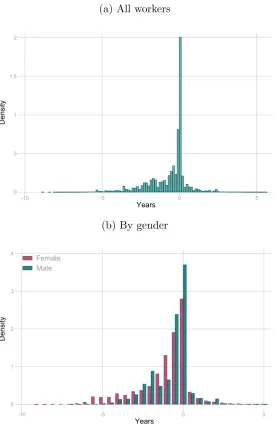
We focus on the change in the full retirement date of older workers on the cusp of retirement before the reform. We definepotential retirees as the full-time employees who could have retired within 3 years under pre-reform rules (i.e. by 2014) and who are directly affected by the reform in the short-run. The 3-year threshold also allows us to focus on a subset of workers with similar age and contribution histories, who at the same time face a diverse enough variation in their full retirement date because of the reform. We will also show how results change when considering shifts in the full retirement date of workers further away from retirement in 2011. Panel (a) of Figure 1.1 plots the distribution of the change in years until the full retirement date forpotential retirees employed in the sample of firms that we describe in Subsection 1.5.2. As already emerged from the heat-maps in Appendix Figure 1.H.3,δθdisplays a substantial variability, with the mean equal to 1.36 and the standard deviation equal to 1.4.
Every potential retiree of type θ experiences the same shift δθ in the expected full retirement date. To construct the firm-level change in the full retirement date, we build a shift-share shock. We weight the δθs by the share of everyθ in the subset of
potential retirees employed in the firm. The firm-level treatment Ti therefore is:
Ti =
X
θ∈Potential retirees
πθ,iδθ (1.2)
πθ,i is the share of type-θ workers among potential retirees employed at firm i in the last quarter of 2011. The πθ,is depend neither on firm size nor on the share of
potential retirees out of the firm’s total workforce. As a consequence, we show that they do not reflect meaningful differences in the broad demographics of the firm. Ti therefore captures the idiosyncratic firm-level shift in the full retirement date of
potential retirees. It also has a straightforward interpretation as the change in the policy parameter that was shifted by the reform. Because of these properties, we use Ti as the treatment variable. In the first part of the paper, where we aim to study the extent of substitutability among workers, we also useTi as an instrument for the number of older workers who delay retirement.
The distribution of Ti for firms that employ at least one potential retiree displays significant variability. The mean is 1.37 and the standard deviation is 1.33 (Figure 1.1, panel b). The variability of Ti decreases with firm size.25 This is one of the
25This is because larger firms employ more potential retirees, so that the distribution of age,
reasons why we focus on small and medium firms, where the variability of Ti is greater.
1.5.2 Empirical Specification and identifying assumptions
1.5.2.1 Empirical specification
To study the effect of the reform we restrict our attention to the sample of firms with a single Contribution Identification Number and with 3-200 employees in the first quarter of 2009 that are active in every year between 2009 and 2015.26 We then
focus on firms that employ at least one potential retiree in the quarter when the reform is passed (last quarter of 2011). Firms with nopotential retirees may not be an appropriate control group, because they have a different demographic composi-tion and are likely to differ along other unobserved time-varying characteristics. We nonetheless show that results are qualitatively similar in the universe of firms in the 3-200 size class. These restrictions leave us with a balanced panel of 61,434 firms.
In this sample, we estimate a difference-in-differences model with a continuous treat-ment and multiple pre- and post-reform periods:
Yit =λi +γt+
2015
X
k=2009
βkT1(k =t)·Ti+εit (1.3)
i indexes the firm and t indexes the year. Yit is the outcome of interest. λi is a firm fixed effect that captures time-invariant heterogeneity across firms, including differences in average outcomes across treatment levels;γt are year fixed effects that control for year-specific shocks common to all firms. Standard errors are clustered at the firm level to address the potential concern of serial correlation across periods (Bertrand et al., 2004). The coefficients of interest are{βT
k}kk=2015=2009 and show how the
treatment Ti affects the outcome of interest in year k relative to the reform year.27 To summarize the results, we also estimate a more compact difference-in-differences regression comparing pre-reform years (2009-2011) to post reform years (2012-2015):
Yit=λi+γt+βTP ostt·Ti+εit (1.4)
We interact the treatment with the dummyP ostt that takes value 1 in years 2012-2015. βT captures the average effect of a 1-year increase of T
i in the post-reform years.
To provide a measure of the extent of labour substitutability, in the first part of
across local labour markets.
26The majority of firms in our size range have a single Contribution Identification Number; some
firms have multiple Contribution Identification Numbers, which however do not necessarily map into different establishments.
27We setβT
additional potential retiree delaying retirement. Specifically, we estimate a version of specification (1.4) where we useTi as an instrument for the numberRi ofpotential
retirees who delay retirement by at least one year relative to the predicted full retirement date under pre-reform rules.28 R
i therefore is:
Ri =
X
j:j∈Potential Retireesi
1(˜δj ≥1) (1.5)
where ˜δj is the observed change in the full retirement date of individualj, i.e. the difference in years between the observed retirement date and the predicted pre-reform full retirement date.
1.5.2.2 Identification assumptions
We leverage variation in the characteristics of potential retirees for identification. The extent to which firms are affected by the reform depends on the distribution of the shares of typesθ among theirpotential retirees (equation 1.2). Identification requires thatπθ,is do not correlate with firms’ unobservable time-varying character-istics (Borusyak et al., 2018 and Goldsmith-Pinkham et al., 2019). In other words, the characteristics of potential retirees employed at a given firm should not corre-late with a firm’s time-varying unobservables. The shares πθ,is depend neither on firm size nor on the share of potential retirees. Thus, we leverage a source of vari-ation that does not depend explicitly on the firm’s broad demographics; we only exploit the variability that stems from idiosyncratic differences across firms in the distribution of gender, age and years of contributions (i.e. in the distribution of types θ) among the narrow set of potential retirees. Evidence that the composition of potential retirees in a firm relates to trends in labour demand would provide a sign of potential threats to identification. Pre-trends as captured by the coefficients
{βkT}k=2011
k=2009 provide suggestive evidence of the conditional exogeneity ofTi. If trends are parallel among differentially treated firms, these coefficients should not be dif-ferent from zero. We also perform placebo and balancing tests to assess the validity of the identifying assumptions.
1.5.2.3 Placebo tests
We assess whether Ti predicts labour demand trends in the pre-reform period by running a series of placebo tests. To this end, we artificially assign the date in which the reform becomes effective to 2010 or 2011, rather than to 2012. We then estimate a version of specification (1.4) on the pre-reform period (2009-2011). We
28We exploit the fact that, everything else being equal, larger shifts in the full retirement date
result in morepotential retireessubstantially delaying retirement. The exclusion restriction requires that the change in the full retirement date affects firms only through a delay in the retirement of
test the effect ofTi on layoffs and new hires, which are the main firm-level outcomes we study in Section 1.7. Appendix Table 1.H.2 shows that a one standard deviation (hereafter 1σ) increase ofTihas virtually zero effects. It is only marginally significant in predicting layoffs when the placebo reform is assigned to 2009. This indicates that firms facing heterogeneous shifts in the full retirement date of potential retirees in 2011 did not exhibit substantially different demand trends in the pre-reform period. Appendix Table 1.H.2 also shows that the standardized share of potential retirees
delaying retirement out of a firm’s employment (i.e. Ri/Ni) predicts trends in labour demand in a stronger and statistically significant way in three out of four cases. This provides ground to the choice of not exploiting variation that captures differences in the broad demographic composition of firms.
1.5.2.4 Balancing tests
We run balancing tests whereby we regress a rich set of firm characteristics at the beginning of the period (first quarter of 2009) on Ti, while controlling for province-sector fixed effects. Appendix Table 1.H.3 shows that the correlations are very weak, although precisely estimated. This holds true when looking at the gender and age composition of the firm. Despite the fact that the reform affected on average women more than men, a 1σ increase of Ti is associated with a decline in the share of male employees of only around 1 percentage point, against an average of 66 per cent. The coefficients relative to the share of young, middle-aged and older workers are 0.00, -0.01 and 0.01, against averages of 0.30, 0.58 and 0.12. We nonetheless show in Subsection 1.7.6 that the results on labour demand adjustments do not change when including the interactions between firm baseline characteristics and year fixed effects as controls. Moreover, column 2 of Appendix Table 1.H.3 shows that the correlations between firm baseline characteristics and Ri/Ni are stronger in almost all cases, further suggesting that firms with heterogeneous demographics differ along many other dimensions.29
1.5.3 Descriptive Statistics
Appendix Table 1.H.4 compares the characteristics of firms in our main sample to other firms with a single Contribution Identification Number, in the same size class and active in 2009-2015. Firms with at least onepotential retireeare on average three times as large as other firms and older. They are more likely to operate in the manufacturing sector and have a higher share of blue-collar workers. Their employees are older, more experienced, have higher tenure and higher daily wages. Appendix Table 1.H.5 shows that potential retirees are older, more experienced, and have higher tenure than other full-time employees working in our sample of firms. They have higher gross daily wages, and are more likely to have a permanent
29For comparabilityT
who are similar along many dimensions.30 Before the reform, employees closer to
retirement were 5 percentage points more likely to be absent from work because of sickness and 1 percentage point more likely to be absent due to work-related injuries or sick leave, suggesting a decline in effort as workers approach retirement.
1.6
Older workers delay retirement after the
re-form
The reform may affect a firm’s labour demand if it prolongs the working lives of older workers. We first investigate the response of retirement choices to changes in the full retirement date by estimating an individual-level version of specification (1.3) on the sample of potential retirees employed in our sample of firms. We use the worker-level shift in the full retirement date as the treatment (δθ in equation 1.1).31 Figure 1.2 shows that delaying the full retirement date by one year causes
an increase in time spent at work and a decline in time spent on retirement.32 A
1-year increase in δθ is associated with 1.5 more months worked and 2.3 less months in retirement in 2015. The increase in months spent at work is smaller than the decrease in months spent on retirement, suggesting that some workers are no longer employed when they start claiming pension benefits. The decline in time spent on retirement is smaller than it would have been had if all workers retired at the predicted post-reform full retirement date (“benchmark”). The difference between the two lines reflects early retirement responses to the shift in the full retirement date.
To quantify the response of retirement choices to the policy, we also use the same treatmentδθ in a cross-section regression where the outcome is the difference between the observed retirement date and the pre-reform predicted full retirement date (Table 1.2). The specification includes age and gender fixed effects. The coefficient on δθ captures by how much workers delay retirement when they face a 1-year shift in the full retirement date. Individuals delay retirement by 7.1 months in response to a 1-year delay in the full retirement date. The response is slightly larger for men (7.51 months against 6.97 for women). These figures are close to estimates in Mastrobuoni (2009) for the US, where a 1-year increase in the normal retirement age causes a 6-month increase in the age at retirement.
30We perform a coarsened exact matching procedure. Matching covariates are: age, gender, type
of contract (open-ended vs fixed-term), occupation, as well as firm’s province, sector and size.
31The regression features individual fixed effects. We also add a vector of controls including
gender and age dummies interacted with year fixed effects.
32Appendix Table 1.H.7 summarizes the results estimating an individual-level version of
1.7
Labour demand responses to the reform
In this section we document how labour demand for co-workers and outsiders changes when there is a shift in the full retirement date of potential retirees em-ployed at the firm. We first present estimates based on specification (1.3); we then summarize the effects by estimating a single post-reform coefficient based on the more compact specification (1.4). Coefficients show the effect of a 1-year increase in Ti. Finally, we present estimates from a modified version of specification (1.4), where Ti is used as an instrument for the numberRi of potential retirees who delay retirement by at least one year. This allows us to provide a more direct measure of the extent of substitutability between employees on the cusp of retirement, co-workers and outsiders.
According to labour demand theory, a drop in demand for other workers caused by the retention of older employees can be reconciled with complementarity between the two types of labour only in the case of an increase in other workers’ wages. We provide the intuition in Appendix Section 1.E, where we develop a labour de-mand model with heterogenous labour and we incorporate different wage formation mechanisms. As we document below, a shift in the full retirement date of potential retirees reduces the demand for co-workers and outsiders. A large wage increase is inconsistent with the evidence in Subsection 1.9.1 that shows a negative effect on the earnings of incumbent co-workers. These results suggest that incumbent co-workers are substitutes for older workers close to retiring. Since the fall in labour demand also involves younger co-workers, our findings provide evidence of substitutability across workers of different ages within the firm. In Section 1.8 we discuss how our results relate to the vast literature on aggregate employment patterns of different age cohorts.
1.7.1 Layoffs
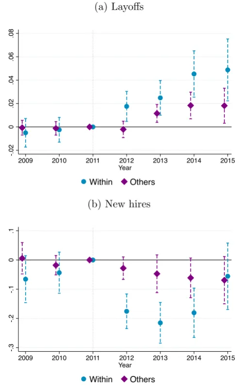
Firms increase layoffs of permanent employees in response to a shift in the full retirement date of potential retirees.33 Panel (a) of Figure 1.3 shows results from
specification (1.3).34 Pre-reform coefficients are not significantly different from 0,
providing supporting evidence to the assumption of parallel trends until 2011. In the post-reform period all coefficients are positive: the effect of an increase in Ti on layoffs is small and not significant in 2012, when most potential retirees would have worked even under pre-reform rules; it then grows and becomes significant in 2013 and 2014, when most potential retirees would have retired in absence of the reform. In 2015, when some of the potential retirees eventually retire, the growth
33Since labour regulations force firms to pay a temporary worker until the contract end date if
he/she is fired for economic reasons, the cheapest way to part from a temporary employee is not to renew their contract. Thus, we focus on layoffs of permanent workers.
0.055 more layoffs - 14 per cent of the pre-reform average number of layoffs per year (0.39). Table 1.3 reports results from the more compact specification (1.4). In the first row it shows that a 1-year increase in Ti causes on average 0.037 more layoffs per year in the post-reform period (column 1); a 1σ increase in Ti (a shift of 1.33 years in the full retirement date) is therefore associated to 0.05 more layoffs, which amounts to 12.6 per cent of the pre-reform average. In the second row we re-scale the coefficients by using Ti as an instrument for Ri. The first stage coefficient is positive (0.21), statistically significant, and the associated Kleibergen-Paap rk Wald F-statistics is large. For every additional potential retiree who delays retirement by at least one year, firms fire on average 0.17 more workers per year in the post-reform period, which amounts to 43.6 per cent of the pre-reform average number of layoffs.
To study the substitutability between incumbent workers, Panel (b) of Figure 1.3 breaks down the effect by workers age. We classify as young the employees of age 35 or below, as middle-aged those aged between 36 and 55, and as old those aged above 55. Layoffs increase in all age groups due to the reform, providing the first ev-idence that firings do not only involve potential retirees. Comparing the coefficients in columns 2 to 4 of Table 1.3 to the group-specific average number of layoffs before the reform, the percentage increase is highest among older workers and lowest among young employees. Focusing on re-scaled coefficients, an additional potential retiree
who delays retirement by at least one year causes 0.086 more layoffs of middle-aged employees and 0.04 more layoffs of old employees; these amount to 43 and 66.7 per cent of the pre-reform averages, respectively.
We further investigate whether the layoffs adjustment on older workers is concen-trated withinpotential retirees or also involves their co-workers (Panel (c) of Figure 1.3 and column 5 of Table 1.3). When focusing only on older workers who are not
potential retirees the coefficients halve, suggesting that half of the response is con-centrated on this category of workers. The firm’s median share of potential retirees
out of older workers is 66 per cent. Thus, potential retirees are not disproportion-ately affected relative to other older employees. Since potential retirees and other older workers earn similar wages, the cost of firing the two types of workers is the same.35 We find that firms trade them off in a similar fashion, suggesting a strong
substitutability.
Panel (d) of Figure 1.3 shows estimates when the dependent variable is the ratio between the number of layoffs in every age group and the respective number of in-cumbent employees at the beginning of the period (first quarter of 2009).36 The
35The cost of layoffs - when ruled unfair by a labour court - is a function of the fired worker’s
wage.
36We therefore estimate this specification on the subset of firms that have at least one employee
coefficients therefore can be interpreted as an approximation of the effect of Ti on the probability of being laid-off. Older workers face a larger probability of being fired than younger co-workers in the post-reform period.
1.7.2 New Hires
Firms more affected by the reform reduce hiring in the post-reform period relative to less affected firms, while there is no evidence that they were on different trends before the reform (Panel (a) of Figure 1.4).37 The pattern of post-reform coefficients is u-shaped: the negative effect emerges as early as in 2012 and peaks in 2013, when a 1σincrease ofTileads to 0.14 fewer new hires, which amounts to a little less than 3 per cent of the pre-reform average (4.79). In 2015 the coefficient is still negative, but not significantly different from 0. This suggests that firms delay hiring in response to the reform; new hires decline in its aftermath and bounce back as potential retirees
become eligible to retire under post-reform rules. Table 1.4 shows that a 1σincrease of Ti on average reduces hiring by almost 0.1 per year (column 1). Re-scaling the coefficients, we find that for every additional potential retiree who delays retirement by at least one year, hiring declines on average by 0.35 unit per year, which amounts to 7.3 per cent of the pre-reform average.
Panel (b) of Figure 1.4 decomposes the effect by new hires’ age. The decline in hiring affects young and middle-aged outsiders to a similar extent. On the other hand, there is no significant effect on older workers, who constituted a small share of new hires in the pre-reform period. For every additionalpotential retiree who delays retirement by at least one year, young and middle-aged new hires decline on average by 0.20 and 0.15 units per year, respectively (columns 2 to 4 of Table 1.4). The decline only concerns new hires employed with temporary contracts (Panel (c) of Figure 1.4 and columns 5-6 of Table 1.4). In 2015 the close to 0 effect on total hiring masks substantial heterogeneity; the effect on new hires under fixed-term contracts is still negative, while it becomes positive for permanent contracts.38
1.7.3 Do firms respond to retirement delays happening in the future?
All workers experience an increase in years left to full retirement, except those who become eligible by the end of 2011.39 We have studied the effects of shifting the full retirement date of workers on the cusp of retirement. In this subsection we test whether firms respond to changes in the retirement date of workers who were less close to retire at the time of the reform. Specifically, we estimate our specifications on the sample of firms that employ no potential retirees, but have at
37Appendix Table 1.H.9 shows the estimates reported in all panels of Figure 1.4.
38Part of this could be caused by a generous package of incentives to foster the use of permanent
contracts that was available to fir