Control Model Development for Packed Bed Chemical Reactors

CONTROL MODEL DEVELOPMENT

FOR PACKED BED CHEMICAL REACTORS

Thesis

by

Rohi

Khanna

In Partial Jilulfi.Ument

of

of

Doctor

of

California Institute of Technology

Pasadena. California

1984

0 1984

Rohit Khanna

iii

To my parents for their support and encouragement

throughout my education and to my wife for her love

iv

This thesis would clearly not be possible without the guidance of my

advi-sor, Dr. Seinfeld. 1 am grateful that he was able to allow me to conduct research

in the areas of my interest without significant restrictions. His assistance is

greatly appreciated. I would also like to thank the National Science Foundation

tor their graduate fellowship that provided much of the assistance for this

research.

Much of the real credit for this thesis should go to my family. Without the

visions and foresight of my parents and without their high expectations this

would never have been possible. Most of all I would like to thank Debbie for her

love and support throughout the time at Caltech and especially on all those

nights when she wished that I could be home but understood that I had to work.

Finally, I would like to thank Dave and Barry for helping provide the outside

interests necessary to keep life stimulating and enjoyable and to retain

v

ABSTRACT

Although control algorithms have been conceived for industrial chemical

systems. their acceptance by industry has been slow due to a lack of direct

experimental evidence of their effectiveness and to volumes of conflicting, or at

least incompatible, recommendations on control structure design. This thesis

provides the basis for a concerted theoretical and experimental program in

mul-ti variable process control structure design for packed bed chemical reactors by

presenting an in-depth control analysis of a practical, multivariable, distributed

parameter system-the heat conduction problem defined by the simple diffusion

equation-using both frequency-domain and time-domain analyses and the

for-mulation, numerical solution, and analysis of a detailed model for packed bed

reactors, along with reduction to a low-order state-space representation suitable

for on-line process control.

The study of the heat conduction system allowed for consideration of

vari-ous control design techniques and the relation between measurement structure

and control system design. This study shows that the choice of measurements

and their locations significantly affects the optimal control design and the

use-fulness of the different design techniques and the importance of an accurate

process model and the necessity of model reduction to a low-order state-space

representation for control structure design and implementation.

The second portion of this study provides a detailed mathematical modeling

analysis of packed bed catalytic reactors that significantly extends previous

stu-dies· in the detail of the model and in the consideration of all aspects of the

vi

general view that modeling simplifications are desired since they lead to a

reduction in numerical solution effort is contested, and it is shown that many

simplifications are no longer necessary with today's advanced computational

capabilities. A unified approach to dynamic reactor modeling is developed and

its importance in the accurate description of dynamic and steady state reactor

behavior, in the investigation of reactor start~up or the effects of process distur~

bances, and in lhe development of an accurate reduced stat~space model for

the design of control structures to stabilize the reactor under various distur~

vii

TABLE OF CONTENTS

Acknowledgement

Abstract

Notation

1. Introduction

1. Objectives of the Current Work

2. Industrial Control Considerations

3. Review of Experimental Control Studies

2. llultivariable Control Structure Design for a Heat Conduction System

1. Introduction

2. Preliminary Analysis

1. Model Red.uctiun.

2. CantrolZa.lTility

3. Root· Locus

3. Tim~ Domain Analysis

1.

qptimal

2. Mod.a.l Cr:mtrol

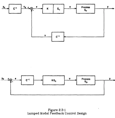
4. Non-Interacting Control

1. Prn"Ject .Dynamic Cl>f111>ensa.tion

2.

3. Set .Pm:nt O>mpensa.tion

4. Inner-Loop .Decoupli:ng

viii

5. Inverse Nyquist Array

6. Characteristic Locus Method

1. Ba.sic System Analysis

1. O:tse !: Measurements z1=0.3, z2=0.7 2. Chse II: Measurements z₁=0.4, z₂=0.6 3. Chse III: Measurements _{2 1} =0.4, z2=0.8

2. Inner Loop .Analysis

1. Qzse I: Measurements Zt=0.3, z2=0.7

2. Chse II: Measurements z ₁ =0.4, z₂=0.6

3. Cb.se III: Measurements~ l;;;:Q.4, ze;;;;0,6

3. Modified Inner-Loop Analysis

7. Control System Performance

1. Case I: Mea.su.rements z 1 =0.2, z2=0.8

2. Ca.se II: Mea.surem.ents z1=0.3, z2=0.?

3. Case III: Measurements zl=0.4, z2=0.6

4. Cb.se IV: Mea.su.rem.ents z ₁=0.4, z2=0.6

8. Discussion of Control Analysis

3. U:athem.aticalllodel of a Packed Bed Catalytic Reactor

1. Introduction

2. Review or Packed Bed Reactor Modeling

3. Model Development for Packed Bed Catalytic Reactors

1. Reactor System

2. Reacf:ion .Ni:netics

3. Formation of OJmplete Mathematical Model

4. Mathematical Rela.tianships

ix

5. N'tl.t71.BriDal Solution

199

1. Solution Techniques

200

2. Orthogonal Collocation

204

3. Model Reduction

20f

4. Numerical Sim:ulaticm

216

4. Model Analysis

223

L Modeling Pa.rameters ₂₂₄

2. Steady-State Beha:uiar ₂₂₉

3. Dynamic Sim:ula.tian.s

230

4. EJ!ects oJ RtuJ.clrYr Dperati:ng Conditions ₂₃₂

5. Radial Ccmcentra.ticm Analysis ₂₃₄

6. Adiabatic Analysis

238

7. ImprYrtance oJ Thermal Well ₂₃₉

8. Dispersion Effects

241

5. OCFE Model Analysis

271

1. Fcrrmulation of oc;:Ji'B' Technique

272

2. Madel Comparisons

279

6. Control Model Development

293

1.

293

2. Model Linea:ri.rza.ticm. ₂₉₆

1.

297

2.

298

300

4. Nu:rnerical Sol~ of the Li:n.earisl:ed Model

302

3. State-Space Si.m:ulatians

304

X

1. Model Discretization

2. Physical Modeli:ng Sim:plifications

1. Horrwgeneous Analysis

2. Quasi Steady State Approzi:ma.tion

3. Negligible EJn.ergy Accumulation in Gas

3. Model Reduction

1. Davison's Method.

2. Marshall 's Method.

4. Discussion of Reduced. Model

4. Results and Di.scUSBi.on of Future Experimental Studies

1. Conclusions of Current Analysis

2. Parameter Estimation and Model Verification

3. Control Model Configuration

4. Control System Design

5. Appendices

1. Computer Programs for Heat Conduction Problem

2. Normalized Packed Bed Reactor Model

3. Radial Collocation of Packed Bed Reactor Model

4. Computer Model of the Packed Bed Reactor

5. Orthogonal Collocation on Finite Elements Model

a.

6. References

xi

A

ft.v.J3v

B

c

c

d

D

F

xii

state matrix

collocation weights for first and second derivative

control matrix

concentration, g-moles I cm5

element ij of measurement matrix C

heat capacity, call g °K

measurement matrix

disturbance vector

radial collocation weights

bulk molecular diffusivity, em 2 _{I sec} activation energy, call g-mole

pressure dependence constants for steam-shift reaction rate

element ij of inner-loop compensator

:r

inner-loop compensator

element of process transfer function

Gp

controller transfer function

interaction compensator transfer function

process transfer function

set point compensator transfer function

heat transfer coefficient between phase i and j, cal!sec em aK

xiii

molar ftu.x relative to molar average velocity

k thermal conductivity

reaction rate constant

Blake·Kozeny constant

diagonal gain element of K

radial (axial) thermal conductivity, cal/sec em °K

K diagonal proportional gain matrix

methanation reaction rate constants, atm-1

low and high frequency compensators

equilibrium constants, atm-2 _{for methanation}

Lagrangian polynomials

L reactor length, ern

controllability matrix

molecular weight of gas, g I g·mole

molar ftu.x with respect to stationary coordinates

-p pressure, atm

total pressure neglecting mole change, atm

closed-loop characteristic polynomial

partial pressure of species i, atm

open-loop characteristic polynomial

Q

r

r

R R

R'

Rg

t

t

T u

Ug

u

v

X

xiv

open~loop transfer function

radial coordinate. em

normalized radial coordinate, r /R1 radial collocation point

reaction rate, g~mole/sec cm3

closed-loop transfer function

radius of thermal well and outer wall, respectively, em

normalized reaction rate

universal gas constant, 1.91:i7 cal/g~mole aK

time. sec

normalized time for heat conduction problem

absolute temperature, aK

control vector

control inputs to heat conduction system

interstitial velocity of gas, em/sec

internal energy

overall heat transfer coefficient between phase i and j, cal/ sec °K

normalized ftuid velocity, u₁/~

volume, cm3

weighting functions

XV

xi mole fraction of species L g-mole if g-mole total

y normalized temperature distribution for heat conduction problem

y output vector

y₀ normalized temperature distribution at t=O

Yd desired normalized temperature distribution

y, normalized mole fraction,

Xt.rx&

z axial coordinate, em

z normalized space coordinate for heat conduction problem

xvi

Greek letters

a

(J

6

1'}

7

"

p

a

dimensionless axial dispersion, oc: Pe;1

dimensionless radial dispersion, oc: Pe;1

moles CO reacted in methanation per total inlet moles

void fraction of bed

dimensionless heat capacity

dimensionless heat transfer coefficient, oc: St

dimensionless heat generation parameters

eigenvalues

Biot numbers

diagonal matrix of eigenvalues

viscosity

constants from radial collocation

normalized radius of therma well,

Ro/R1

dimensionless heats of reaction

density, g/cm3

dimensionless reaction coefficients

dimensionless pressure drop,

Pz=LIPz=e-

normalized time, (t ·il~o)IL

normalized temperature.

TIT

xvii

Subscripts and Superscripts

0 value at inlet

b reactor bed

f value at outlet

g gas

h heat

m mass

M methanation reaction

r radial

s solid catalyst

s

t thermal well

w cooling wall

z

based on inlet conditions

steady state

Chapter 1

-2-One of the major difficulties in the application of advanced process control

theories to industrial chemical processes is the lack of complete understanding

of the chemical process and the inability to predict system behavior in the

pres-ence of unknown and uncharacterized disturbances. This difficulty is

com-pounded by physical and chemical interactions or nonlinear coupling of the

pro-cess variables. Although complex control algorithms have been conceived for

industrial chemical systems, their acceptance by industry has been slow due to

a lack of direct experimental evidence of their effectiveness and to volumes of

conflicting, or at least incompatible, recommendations on control structure

design. Significant research efforts are necessary in duplicating industrial

processes in a research setting and providing a unified approach to the

mathematical modeling and control structure design.

This thesis provides the basis for a concerted theoretical and experimental

program in multivariable process control structure design for packed bed

reac-tor systems. Along with the detailed design and construction of both a kinetics

and pilot-scale control reactor {Strand, 1984), this work presents the necessary

prerequisites to a substantial effort in the study of the applicability of process

control theory to a laboratory- or pilot-scale industrial chemical process. In

view of these objectives, this thesis is divided into two major sections:

- an in-depth analysis of a practical. multivariable, distributed

parame-ter system-the well-defined beat conduction process defined by the

simple diffusion equation-using both frequency-domain and

time-domain analyses and

-the formulation, numerical solution, and analysis of a detailed

low-order state-space representation suitable for on-line process control.

The first section of this work, the analysis of the heat conduction problem,

is presented in Chapter 2 and is a self-contained presentation of many of the

control aspects of a multivariable, distributed parameter system (Khanna and

Seinfeld, 1982). Although this heat conduction system is much simpler than the

packed bed reactor, a considerable amount of insight into control structure

design can be obtained from this process since the control aspects are not lost

in the complexity of the mathematical system as they may be in an initial

detailed control study of the experimental packed bed reactor. In particular, an

analysis of a number of multivariable process control strategies, including

non-interacting control, optimal control. inverl:!e Nyquist array, and characlerislic

locus techniques, is carried out theoretically on a one-dimensional. two-input

heat conduction system. The potential improvements in control performance

through the usc of extra measurements and through the appropriate selection

of measurement locations is assessed and a new non-interacting control

stra-tegy, termed inner-loop decoupling, is developed.

The remainder of this thesis centers on the complete dynamic modeling

analysis of a packed bed reactor, along with reduction to an accurate low-order

state-space representation suitable for control studies. According to Jutan et al.

( 1977). this is

-4-In view of these comments, this study allows accurate description of dynamic

and steady state reactor behavior for process optimization and design. for the

investigation of reactor start-up or the ef:J'ects of process disturbances, and for

the analysis and design of control structures. Various common assumptions

and model structures are considered, and the appropriate numerical solution

techniques are discussed. This analysis is not intended to be specific to any

par-ticular packed bed reactor system but rather to present a detailed study of

modeling techniques, assumptions, and solutions and to develop a unified

approach to dynamic reactor modeling and control model development. The

work significantly extends previous studies in the detail of the mathematical

model and in the systematic consideration of all aspects of the model

-5-1.2 INDUSTmAL CONTROL CONSIDERATIONS

Until only recently, the process control industry has been dominated by

applications to mechanical or electrical processes where systems are generally

well-defined and numerically simple due to minimal nonlinearities and relatively

simple physical characteristics. Even so-called 'modern' control theories

developed in the 1960's have only played an important role in fields such as

robotics and the space program. Their applicability to complex industrial

chem-ical processes which are inherently burdened by nonlinearities, large time

delays, and distributed parameter behavior has been extremely limited in spite

of an enormous effort by researchers. Although significant theoretical efforts

have been made by many research groups in the development of control

algo-rithms for ill-defined distributed parameter systems as are common in the

chemical industry, these efforts have not found wide application in actual

indus-trial problems. Thus during the past twenty years, a significant control 'gap' has

developed between process control theory and practice (Foss, 1973; Seborg and

Edgar, 1982).

Due largely to increased costs for energy, increased governmental safety

and environmental restrictions, and increased foreign competition, significant

efforts are now being made by industry to modernize and automate production

facilities with a major emphasis on integrating energy requirements and

improv-ing throughputs and system performance (Ray, 1981). Additionally with the

major improvements and general acceptance of computers suitable for on-line

control, attempts at applying sophisticated control theories are only now

begin-ning. One of the conclusions of the discussion on the problem of the control

'gap' between academic theories and practice is that there exists a ·pressing

need for careful, systematic studies of the design and implementation of control

behind the current theoretical and experimental program for which this thesis

provides a basis.

Several steps are necessary prior to developing and testing control

stra-tegies. These include the design and construction of a pilot-scale system

pos-sessing much of the modeling characteristics and control difficulties of the

actual industrial process, the development of an accurate mathematical model

for process design and analysis, and the reduction of the full model to one

suit-able for control structure design and on-line control. The first of these steps

was performed by Strand (1984), and the latter two steps are the concern of this

current work. A packed bed nonadiabatic chemical reactor was selected as the

chemical process to be studied due to its complexity and inherent control

difficulties and its extensive industrial importance for carrying out exothermic,

gas phase reactions.

Upon completion of these preliminary research efforts. the elements of the

control structure:

• the measured variables,

• the manipulated variables,

• the control configuration connecting the measured and manipulated

variables, and

• the control logic governing the behavior of the manipulated variables

can be considered. In particular, it is important to determine control

struc-tures that make optimal use of the availiible measurements in the chemical

pro-cess. Although in general there may be quite a few measured variables available,

they may not be the variables of most concern, and these variables may need to

be reconstructed using the process model. An example of this is the

-7-outlet concentrations may need to be estimated. Further problems with

meas-urements result from various random and systematic errors or noise in the

measurements and long delays due to the complexity of the chemical or

physi-cal analyses.1 _{The use of an accurate process model can in many cases minimize}

these diffl.culties by allowing prediction of some unavailable measurements, by

improving the knowledge of the system performance through simulations, and

by allowing design improvements to the process.

Thus the central role played by dynamic and steady state models in the

design and optimization of chemical processes and in the development and

application of control strategies justifies considerable effort in their

develop-ment. The philosophy of this modeling work is presented by Foss ( 1973),

'Forms

ot

differential equations to empirically or experimentally derived transfer functions. The forms of the models may not be selected arbitrarily: they are determined in part by the control objectives and the type of control analysis to be pursued. In short, process modeling is a substantial and crucial task, and by no means routine. .. . The operation of control systems of modern design also requires estimates of the process states used for control. This requires a process modeL perhaps different than that used for design calcula-tions, and a means of rapid solution of the model equa-tions."

The work presented in this thesis is intended to minimize the diffl.culties

associ-ated with process modeling by providing an accurate unified approach to the

model development for packed bed chemical reactors.

-8-1.5 REVIEW OF EXPERIIIENTAL CONTROL S'I'UDIES

Several experimental laboratory-scale packed bed reactor systems have

been studied in terms of control considerations. Table 1.2-1 outlines some of

the work done by several groups that have made significant contributions in this

area. Their work is by no means the extent of control applications for chemical

processes (there is much published work on the control or separation processes

and other reactor configurations) but is the major extent of published

experi-mental application of control techniques to packed bed reactors.

The Denmark group (Clement and Jorgensen, 1981; Clement et al., 1980;

Hallager and Jorgensen, 1981; Sorensen, 1977; Sorensen et al., 1980) considered

an adiabatic pilot-plant chemical reactor with the reaction between oxygen and

hydrogen over an alumina supported platinum catalyst. Initial dynamic

model-ing and experimental studies were carried out by Hansen and Jorgensen (1974,

1976ab) and by Sorensen (1976). The group considered various reactor and

control models and investigated control strategies based on optimal control.

direct Nyquist arrays, and the self-tuning regulator.

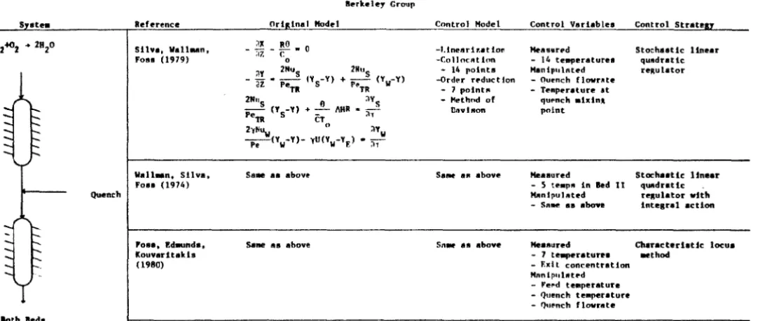
The Berkeley group (Foss et al., 1980; Michelsen et al., 1973; Silva et al.,

1979; Vakil et al., 1973; Wallman et al., 1979) studied the same hydrogen/oxygen

system but used a two-bed reactor structure with an interstage quench stream.

Again the beds were taken as adiabatic, and various control strategies were

de-vised. The first control studies by Silva et al. (1979) and Wallman et al. (1979)

considered the control of the quench fiowrate and temperature using

tempera-ture measurements and a product concentration estimator using the stochastic

linear quadratic regulator and multivariable integral control. The latter work

by Foss et al. (1980) uses the tlowrate and temperature of the quench stream

tempera-

-9-ture using the characteristic locus method of control system analysis. A major

significance of their work was the consideration of the large number of available

measurements and the appropriate choice of control contlguations.

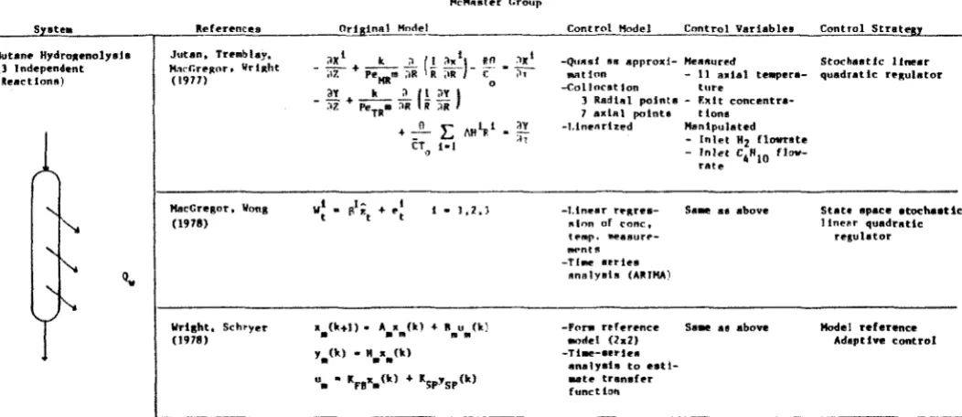
The McMaster group (Jutan et al., 1977; MacGregor and Wong, 1978; Wright

and Schryer, 1978) considered the hydrogenolysis of butane carried out over a

nickel on silica gel catalyst in a nonadiabatic packed bed reactor. The work by Jutan et al. ( 1977) provides an excellent foundation for packed bed reactor

modeling and control studies for multiple reaction systems by specifically

con-sidering the state-space model development, the parameter estimation and

sto-chastic disturbance identification, and on-line linear quadratic control. The

ear-lier work by MacGregor and Wong (1978) and Wright and Schryer (1978) deviated

from the mechanistic approach to reactor modeling taken by most studies

where models are developed by careful consideration of the important chemical

and physical phenomena occurring within the process. They considered the use

of statistical methods to identify process transfer functions from empirical

input/ output process data. They then applied a model reference adaptive

con-troller and a state-space stochastic linear quadratic regulator.

Finally. the dynamic behavior of an autothermal reactor with internal

countercurrent heat exchange using the steam-shift reaction was modeled by

Bonvin (1980) and Bonvin et al. (1979, 1980). Modal control using state

feed-back was found appropriate for stabilizing the reactor around an unstable

f)pnMRrk Group

Syat8 leferencu Orleln~l Hodel Cont_':£!._!fodel Control Variables Control Stnteu

H

2 + o2 + 2H2o

Acllabattc

Sorensen (1977) Cleaent. Jorf(l!'nsen, Suren•n•n (191!0)

Cle..nt • JorR.ensen (198!)

RallaAf!r. Jor~ten­

' " " (!'Jill)

2

-~+--l_U_!t~.o

;l7. PeMl" ;)Z2 C

0

2

- ~ + _ I _ ~ - ~~ (~-Y )

:•~ Perz" az2 r"TR w

Same 111 s above

- fl_ fiHR • _;l!

CT ;Jt

0

x(t) • A(q- 1)x(t-1)+8(q-l)u(t-d) +e(t)+c or

Kl(t) • ·~(t)OI + el(t)

Table 1.2-1

- Cot }:watton (4-A rotnts) - 1~tne~trized

Snmr AS above

Mtaftsured

- 1l t""'P"rature - 6 o₂ concentration - Tnt<1l flow-rate Hanhmlated

- J-"l'f"tl teaperat1.1f't!

- o₂ feed

concen-tration - Tntnl ftovrate

s .... _. .as above

- te.1At 8CJUATeR Same AS above !dent H lent ton

- Tf.e series

Model

Summary of Published Research on Packed Bed Reactor Control

Stochastic linear qu•dratlc reRulator

Direct Nyquist array

Hfl<lll ... u -tuntna

r<Jiulator (LQR)

I

~

Syate.

11

2..02 + 2H2o

~~

....

----

~

loth lleda AUabattc

Quench

Reference

Silva, Vallun, Fou (1979)

Wall•n, S!lva, Fon (1974)

Pose. !d.unda.

Kouvar1taltls (1980)

ortgina I llod•d

rlX RO • c - ;iZ - co

2Nu

~ • _ _ s (ts-Yl

- oZ PeTR

Berke t ey Group

2Hu 5

+ - p - {Yw-Yl

~TR

211u5 Y) + ...!!._ AIIR

- - (Ys- -PeTR CTo

avs -~

2)'~"w(Y -Y)-yU{YW-YE) Pe W

Sa.e aa

above-Salle aa above

avw

-~

Control Hodel

-tlneari7.atlor~

-Co II ocRtl""

- 14 points -Drdt'r r .. ductlon

- 1 point" - l!t!thnd of

D-nvlfaon

Sa• att above

Sn.- as abov~

Table 1.2-1 Continued

Control Variables

Measurpd

- 14 te,..,eraturea ManipulAted - {luench flovr•te

- Te•perature at quPnch •lxinA roint

Heaaured

- 5 tell!'~ in lied It

Man!pu!At..d - Sa.e aa above

Me•attred - 7 te....,raturn - F.xl t concentration Mnntpulltt .. d

- r.,.d te,..,erature

- Quench te....,rature

- Qu•nch flovrate

Control Strateu Stochastic linear

quadratic

re~~tulator

Stoc:haettc Unear

q~drattc

re11ulator vtth integral aetlon

McM~tat~r Group

SysteM Jlef.,r•ncu Original Hodel Control Hodel Control Variableo Control Strategy I

lutan• Hydro11HolyaJa

0 Jndepen4ent Reactions)

0..

lfonadta .. t tc

Jut an • Tre-mb 1-av.

H~rr.re~or. Wrt~ht

( 1977)

MacGregor, Wong (1'178)

Wright, Schtye1" (1978)

ax 1 t. ~ ( 1 a.1J ~~~ ~x 1

- TfZ + PeHRm ;:;R R ;tjt - ~ • ; l l

at k altav}

- ~z + Pen• :>R i! :lR

+-!-

E

0

wl • ciA + 1

t " P.t .. t i - 1,2,}

X

.

..

.

..

y

. .

..

"• • KFB"• (k) + K;pYsp (It)

ay

-~

-Qmtsf !ls .llppro-xi-Hettftur~d

IMtion - 11 adal

t•~era--Collocllt ton ttn-e

J Ra~id pointe - 1\x!t concentra-7 axlltt pointe

-l.in•Arhed

-t.tne-ar t'e~re-s­

Rion or cone,

ttt"'''4 ~~~easur~­

MPnts -Ttae- •trie-s

analysis (AUMA)

-Fo-rw Tl!fe-rence

...,del (2z21 -Tt.e-•erte-tt

ana I yah to eati-ute- transfer functt()tt

tiona Manipulated - In I et 112 floon:ote - lnl<?t c₆11₁₀ f l

-rate

Sa• ae above

SaM ae above

Table L2-1 Continued

Stochaatfc ltnear quadrat tc rekulator

State space atochaatic

II near quadratic

r~1uletor

Model reference

Adaptive control

Chapter 2

:MULTIV.ARIABLE CONTROL STRUCTURE DESIGN FOR

-

14-2.1 INTRODUCTION

Classical process control techniques were largely developed on a trial and

error basis, with the theoretical concepts developed later to substantiate the

empirical results. The classical controller was based on a input,

single-output (SJSO) system with three types of possible control action-proportionaL

integral, and derivative-based on the feedback error. Although design

tech-niques such as root-loci, Bode diagrams, and Nyquist plots led to empirical rules

for setting the appropriate amounts of control action, these methods were

lim-ited to SISO systems. Since most processes have multiple inputs and outputs,

additional considerations became necessary, due to the failure of single-loop

analysis for interacting loops. Since frequency-domain methods dominated con-trol system design in the scalar case and led to relatively simple concon-trollers, it is

not surprising that considerable effort went into extending these methods to the

multivariable case. However, direct extension of scalar frequency-domain

pro-cedures was not possible, and major modifications of the existing theories were

necessary to meet the design objectives. Furthermore, design complexities were

often enhanced due to the additional objective of noninteraction. Nevertheless,

several excellent frequency response procedures were developed in the late 60's

and 70's, led by the work of Rosenbrock, MacFarlane, and Kouvaritakis.

At the same time, ''modern" control techniques were developed. These

methods rely on an exact knowledge of the system state, which is reconstructed

from a finite number of measurements using current theories in optimal

filter-ing, smoothfilter-ing, and estimation. The ideas have been extended to account for

modeling and measurement uncertainties and inaccuracies. Although these

''modern" methods, which rely heavily on variational calculus and dynamic

pro-grarn.ming, generally lead to a more complex control structure, they are less

-

15-control objectives, such as the minimization of the variance in the state vector.

This chapter describes an in-depth analysis of a practical. multivariable,

distributed parameter system using both frequency-domain and time-domain

analysis. As a typical distributed system, a one-dimensional, heat conduction

problem is considered. The process is described by the difiusion equation

tJ2y(z,t)

az

By(z.t)

Bt (2.1-1)

where the temperature distribution, y(z,t). is dependent on the space coordinate

z. which is normalized (0.0

<

<

sys-tern, and on time, which is normalized so that the coefficient corresponding to

the thermal difiusivity is unity. For simplicity, the controls u₁(t) and u₂(t) are

taken to be the heat fiuxes at z ""' 0 and z ""' 1. Thus the initial and boundary

conditions are

y(z,O)

=

By(z.t)

j

=

Clz •=O

By(z,t)

j

=

az

(2. 1-3)

Although this heat conduction process is a relatively simple control

prob-lem due to the simplicity of the model and ease of obtaining measurements. the

analysis leads to conclusions that can be extended to general, multivariable

control theory. Actually the system is an excellent choice, since Equations (2.11)

-(2.1-3) can be solved analytically to give the temperature distribution for any

control action. Thus model reduction and control design techniques can be

applied to the reduced system and compared with the actual process model.

Additionally, the heat conduction system is a highly interacting process with

implicit transportation lags.

-

16-can be performed. Since most frequency-response techniques require a

low-order, lumped, state-space representation, model reduction is an important

step in the analysis. Section 2.2 discusses the model lumping and reduction

using exact techniques. Additionally, an analysis of output and system

control-lability, along With a multivariable root-loci analysis, is presented. Much insight

can be obtained from these preltminary considerations.

Section 2.3 discusses the time-domain analysis of both the lumped and

dis-tributed models of the system. Both optimal feedback control and modal

tech-niques are discussed in detail, along With derivations of the control schemes.

Since much work has been published on the application of optimal control

theory to the single-input, one-dimensional heat conduction problem and since

little additional complexity 1s introduced in the optimal analysts by adding

another control. this aspect is not dealt With in detail.

Section 2.4 considers non-interacting control. Since a major difficulty in

multivariable, feedback control design arises from the steady state and dynamic

interactions that occur between the various input and output variables. it is

usually desirable to reduce these interactions. If they can be reduced

sufficiently, single-loop control theories can be applied directly to each of the

non-interacting loops. The technique of perfect, non-interacting compensation

is attempted for this purpose. However since such compensation is in many

cases impractical or excessively complicated, other methods that only eliminate

steady state interactions are also considered. Finally, a new method, that uses a

relatively simple control structure to eliminate all steady state and dynamic

interactions, is considered. This procedure, called inner-loop decoupling, makes

use of extra available measurements through an inner-loop structure.

frequency-responsA analysis are also studied. Section 2.5 discusses the application of

Rosenbrock's (1962) inverse Nyquist array technique, which is an extension of

the classical Nyquist stability criterion. Section 2.6 analyzes the heat

conduc-tion system using the characteristic locus method. The analysis is based on the

latest refinements of the technique originally introduced by Belletrutti and

MacFarlane (1971). The current work provides a systematic approach for

designing a proportional-integral controller with the best compromise of system

stability, interaction, integrity, and accuracy.

Section 2.7 presents an overall analysis of the control system performance.

Using computer simulations of the responses of both the lumped model and the

actual system to step input changes, the effectiveness of the various control

designs are compared. This analysis leads to conclusions about the model

reduction and design techniques that can be extended to general, multivariable

-

16-2.2 PRELllliNARY ANALYSIS

Difficulties arise in the control system design of distributed parameter

sys-tems because of state variations in both time and space. The thrust of many of

the feedback control design techniques for distributed systems is to reduce the

system to a lumped one and then to take advantage of the many theories

avail-able for lumped parameter control design. However, problems arise in that all

of the analysis performed on the lumped system is dependent on the method

and accuracy of the reduction. Although considerable model reduction is

neces-sary to reduce computational complexities in the design procedures, excessive

or inaccurate reduction can lead to a system whose behavior is quite different

from that of the original process.

2.2.1 Yodel Reduction

To obtain the lumped parameter model for a system described by partial

differential equations, many efficient techniques are described in the literature.

In particular, much work has been published on various lumping strategies for

linear diffusion equations. A particularly useful means of treating both linear

and nonlinear partial differential equation systems is the method of weighted

residuals along with other pseudo-modal techniques, such as finite element

methods (Norrie and DeVries, 1973) or the use of spline functions (Finlayson,

1972). The method of weighted residuals is comprised of the following basic

techniques, depending on the choice of the weighting function (Prabhu and

McCausland, 1970; Ray, 1961):

a. Galerkin's Method (Lynn and Zahradnik, 1970; Newman and Sen,

-

19-b. Method of Subdivisions

c. Method of Moments

d. Method of Collocation (Finlayson, 1972)

e. Least Squares Method.

Although these techniques are quite powerful, Mahapatra (1977) points out that

solutions using the method of weighted residuals often require considerable

effort to determine the set of orthogonal coordinate functions and a high·order

lumped model for accurate results. To eliminate these difficulties, spatial

discretization techniques (Leden, 1976; Mahapatra, 1977) are often quite useful

tor linear ditfus10n systems, since they retain the physical characterist1cs of the

system. However, they too often lead to high-order lumped models.

Thus to improve the accuracy and reduce the order of the model, it may be

best to use an exact reduction technique. Since the heat equation is governed

by a parabolic equation, exact lumping can be performed using a Laplace

transform in time or through a modal analysis. The latter, which is simply an

application of the separation of variable solution procedure, is quite attractive

for systems which can be made self-adjoint, since the technique leads directly to

the eigenvalues and eigenfunctions (modes) of the system. If the eigenvalues

are real, discrete and well spaced, the modal representation is a convenient

method to reduce the order of the system, since only the dominant modes need

be retained for design purposes.

Both the Laplace transform and modal analysis techniques were applied to

the one-dimensional heat conduction problem. Other techniques have been

dis-cussed in detail in the literature. Although the methods can be shown to lead to

equivalent results, the modal analysis leads directly to a lumped, state-space

cited by Prabhu and McCausland (1970), but the technique is well suited to the

linear diffusion problem because time and space variables are easily separated

and an analytic solution is possible.

Consider the system described by Equation

(2.1-1),

Taking the laplace transform with respect to time gives:

sy(z

s)

, dz2 ,

which has the solution

y(z,s) =A sinh ...JSz

+

dy(O,s) _ ( )

- -u1 s

dz dy(l.s) dz = u2(s) .

the solution in the Laplace domain is

y(z,s) = GJ'(z,s)u(s).

where

T _ [ ] _ fl cosh( 1-z)-Vs cosh zv'S

J .

Gp- g1(z,s) 'g2(z,s) - v'Ssinhv'S ' v'ssinh..JS

(2.2-1)

(2.2-2)

(e.z-s)

(2.2-4)

(2.2-5)

(2.2-6)

Thus a distributed transfer function representation is obtained, from which a

simple feedback control strategy can be env{sioned

(Figure 2.2-1).

closed-loop distributed transfer function is

y{z,s)

Yd(z,s) (2.2-7)

However in general, measurements will only be available as discrete points. If

-

21-Figures 2.2-2 and 2.2-3 with

(2.2-8)

Note that Figure 2.2-3 is equivalent to Figure 2.2-1 with Gc(z,s)

=

Gc(s)A

Using contour integration to invert Equations (2.2-4)-(2.2-6), the

time-domain representation of the solution can be obtained. The inverse of g,;(z,s) is

the sum of the residues of estg1(z,s). Each g,(z,s) has an infinite number of

sim-ple poles at Sn

=

, n

=

=

the numerator and denominator of estg,(z,s) about s0

=

1. 0 at s0. The residues at Sn are obtained by Taylor expanding sinh ....; s about

sn

and applying residue theory. This results in

- 1!2t,

g₁(z.t)

=

2:

n=l

g₂(z,t) ::::: 1.0 +

~

(2.2-9)

n=l

Then using convolution theory. the t1me-domain behaVior is directly related to

the control action:

t

y(z,t) :::::

fo

=

Since the time-domain results are obtained as an infinite series of

exponen-tials with eigenvalues Xn

=

, the Laplace-domain behavior can also be

represented as an infinite series with y(z,s) being described by Equation (2.2-4)

along with the following:

GJ(z,s)

=

[.L+

f:

.L+

f:

l .(

S n=l s-Xn s n=l s-Xn

Then if the series can be truncated after the first few terms without excessive

-22-However since separation of variables for the one-dimensional heat

conduc-tion system leads to a self-adjoint operator With real. discrete eigenvalues,

modal decomposition is attractive for this system. The problem can be

redefined using the Dirac delta function:

By1~·t)

~~~,t)

+

~(z-o)ut(t)

z

o-,

z

=

~~.t)

=

o .

(2.2-12)

It can be proven that this change is rigorous by integrating Equation (2.2-12)

across the infinitesimal intervals 1-< z < 1 +and

o-

,.o+

,.o+

~y)

o-~-

,.o+

;

0_ ¥t-dz =

Jo-

fo-

Jo-

Thus

But

~"}

=

~i

(2.2-12) is equivalent to that described by Equations (2.1-1)- (2.1·3).

The space and time variables can then be separated by assuming a solution

of the form

..

y(z,t) ::: ~ an(t)~n(z)

n=O

..

t5(z-D)u₁(t) +o(z-1)u2(t)

=I;

n=O

A!ter substituting into (2.2-12) and simplifying, the equations become

-23 ~

n

=

z=O

-'-:;;...;-=

z

=

By choosing the separation constant as -An,

n=O, 1, 2, ... . (2.2-16)

Clearly (2.2-16a) is a self-adjoint differential equation that can be solved to yield

(2.2-17)

after application of the boundary conditions from (2.2-15). Because (2.2-16a) is

a homogeneous, self-adjoint differential equation With homogeneous boundary

conditions, the eigenfunctions, Equation (2.2-17), are orthogonal. It is

con-venient to choose the arbitrary constant

An

orthonormal, i.e.,

1

fo

=

The appropriate choice of An leads to

{ 1.0

Y'n(Z)

=

-.n_

n=O

n= 1. 2 .... (2.2-19)

Then by application of the orthogonality of the eigenfunctions

1

e.n(t)

=

fo

Thus

1

bn(t)

=

fo

=

n=O n=1,2, ...

(2.2-21)

(2.2-22)

Since the eigenvalues,

7\n

=

sys-tern can be accurately represented by the first few eigenfunctions, n

=

The process model can then be obtained as an Nth-order lumped state-space

representation with theN+ 1 states a0, ... , aN.

X(t)

=

=

1 1

'-'Z

-..JZ

(2.2-23)

The resulting feedback control system can be drawn in block diagram form

(Fig-ure 2.2-4)

In theory, the control scheme of Figure 2.2-4 (and of Figure 2.2-1) requires

the complete temperature profile, y(z,t), of the system. However, Ray (1981)

-25-L measuring y(7,,t) at many points i

=

smoothing technique to approximate y(z,t),

ii. measuring y(Zt.t) at a few points and using a state estimator to

esti-mate y(z,t),

iii. or measuring y(zt.t) an N+l spatial points and letting

y(t)

=

C= (2.2-24)

Then y(t)

=

=

keep C nonsingular.

Actually it is possible to control the system by taking measurements at M points,

where M

<

points on the outputs rather than on the states, since the N+ lth-order state

vector x:(t) cannot be obtained uniquely with M

<

Regardless of the technique for estimating y(z.t), the appropriate transfer

function representation can be obtained by converting to the laplace domain.

With Yo (z)

=

x(s)

=

=

or with measurements at M distinct points:

-26-Thus the lumped parameter system process transfer function is given by

(2.2-27)

2.2.2 Controllability

The distributed system has been lumped through an N eigenfunction

decomposition. Before attempting to design a control strategy for the lumped

system, an analysis of system and output controllability is necessary.

Although the concept of controllability is formally defined in many

refer-ences (Brockett, 1970; Douglas, 197Z; Lee and Marcus, 1967; Ray, 1981), it is

con-venient to consider a system completely controllable if some control action

exists that will take the system from any given initial state to any specified final

state in finite time. The necessary and suffi.cient condition for complete

control-lability of the system described by (2.2-23) with N-1 states and two controls is

that the controllability matrix

It:

' 1

..JZ

1

-"2

0

-(_,.2~-JZ

(2.2-28)

has rank N-1. Since

It:

controll-able. Thus the two controls u1 and u2 are capable of influencing all of the states.

However, the lumped. analysis will be based on k measurements. Thus a

more important concept is that of output controllability, i.e., the controls must

-27-4'

=

[CBI CABI ...

l

must have rank k for the system to be output controllable. It can easily be

shown that, for the heat conduction system, output controllability is assured if

no two measurements are taken at the same point.

It can be concluded that, for k distinct measurements, the lumped,

one-dimensional heat conduction system is completely controllable with heat fiux

control at z

=

=

can be applied to the state-space representation of the system. However, it

should be recalled that this analysis or controllability is dependent on the

accu-racy of the model reduction and lumping. Although the approximate lumped

parameter system has been shown to be completely controllable, the actual

dis-tributed system may indeed be only partially controllable. Additionally, care

must be taken in making conclusions from this type of analysis, since no

con-sideration of the physical constraints of the system have been made.

2.2.3 Root-Locus

The concept of root-locus analysis is basic to classical control system

design for single-input, single-output processes. The root-locus diagram is

advantageous since it describes the character of the response as the gain of the

controller is continuously changed, by allowing rapid determination of the roots

of the characteristic equation. Although scalar root-locus techniques are

well-known, the multivariable root-locus problem is relatively new. Kouvaritakis

(1978), Kouvaritakis and MacFarlane (1976ab), and Kouvaritakis and Shaked

( 1978) describe the technique and discuss the analysis of system zeros.

The objective of the root-locus method is to investigate the behavior of the

-28-form

Gc =

sys-tem, the process transfer function was shown to be Gp

=

characteristic equation is then (Hsu and Chen, 1968)

(2.2-30)

where P₀ (s) is the open-loop characteristic polynomial and Pc (s) is the

closed-loop characteristic polynomial. Then if we detine

si-A -B

z(s)

=

C Om,m

the n-m-d closed-loop characteristic frequencies1 _{will tend toward the roots of}

z(s)

=

two-control. 3rd-order, heat conduction system, there is one finite zero and two

infinite zeros if CB has full rank. If CB has lost rank, all three zeros will be

infinite. This occurs for the following choices of measurement locations:

Z1 0.20 0.33 0.40 0.60 0.67 0.80

z

Thus for any combination of outputs other than these, there will be one finite

zero given by z(s)

=

8

=

2_(c-a)

V2(ad-bc)+(a-c) (2.2-32)

-29-This root is finite for all z1 and Za other than those listed above, since the

denominator of Equation (2.2-32) is then nonzero.

The root-loci for the system are the loci of the roots of the characteristic

equation

+4k(ad-bc)]s +Brr2~k(a-c)+Brr4] (2.2-33)

as k varies from 0 to cc. Obviously, the poles (k

=

=

-rr2 _{and -4rr}2 _{independent of the measurements. As k approaches infinity,}

(2.2-33) reduces to

~(ad-bc)s + (a-c)s + 4rr2(a-c)

=

which is equivalent to (2.2-32) above.

(2.2-34)

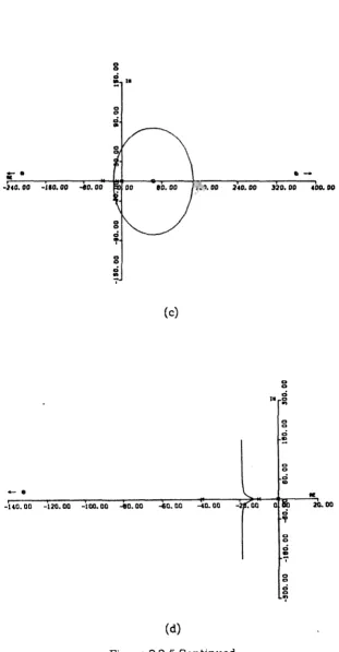
Figure 2.2-5 shows the root-loci for various measurement locations. Both

symmetric and unsymmetric cases were studied. For the symmetric cases, the

root-loci remain stable (in the left-half plane) at high gains for z1

s:

whereas, the loci become unstable at high gains lor 0.33

<

expected due to the large lag time between the control action at z₁

=

effect on the output. The symmetric cases with

z

z

z

>

and z₂

<

except that the locus beginning at -1r2 approaches +oo rather than -co. Thus

such a system is less stable.2 Additionally from the root-loci analysis. the

-30-responses for the (0.2,0.8) case are expected to be non-oscillatory; whereas, for

all other cases, oscillations are expected at moderate to high gains.

It can be concluded that, for symmetric measurements with z1

<

gains. Thus a proportional controller may provide adequate control action.

Since the other cases lead to instability at high gains, more complicated control

Yd(z,s) i'L >(

-E'(Z,S)

-

31-Gc(s) u(s) -... Gp(Z,s)

Figure 2.2-1

Distributed Feedback Control Design

Measuring Device

Figure 2.2-2

Process

Gp(Z,S)

Feedback Control Strategy with N Discrete Measurements

y(z,s)

-32-Yd(z,s)

A

~

A

Figure 2.2-3

Modified Feedback Control Strategy with N Discrete Measurements

Yd(z)+/0\ E(Z t)

Gc(z,t) u(t)

x=

Ax

'<:1

'

=

Cx(

-Figure 2.2-4

-33--.

-·

-uo. oo -no. oo -100. oo -10. oo ...o. oo -•o. oo -20. oo

(a)

-·

-·

I .. 0

II

..

•

...

;

•

...

•

•

-..

..

"'

.. ..

...

•

...---~-,,-.,----,---i--..---. ... --....--~-+-

....

0

..

,.

..

Figure 2.2-5

Root-Loci Diagrams for Various Outputs

a. (0.2,0.8) b. (0.3,0.7) c. (0.4,0.6) d. (0.4,0.8)

...

8

! ..

g

-34-

·--1to. oo -JJo. oo -eo. oo 011 2411. 110 J:lO. 011 tOO. 110

(c)

D D

II

..

...

"'

"'

..

!:

..

"'

..

..

-·

•

-uo. oo -120. oo -too. oo -eo. oo -60. oo -to. oo

..

0

"'

..

..

-.

"'

..

..

..

.., I

(d)

2.3 TlME-DOM.AlN ANALYSIS

The time-domain approach for control system analysis utilizes the

differential or difference equations directly rather than using transfer functions,

as in the frequency-domain analysis. Although the time-domain technique is

actually older than frequency response techniques, its development was slow

due to the difficulty of making calculations in the differential domain. :rhe

emergence of digital computation as a widely accepted tool led to a resurgence

of interest in time-domain analysis. In particular, the techniques of state

esti-mation, optimal control, modal control, and adaptive control rose to the

fore-front of research. Although these methods have a strong theoretical basis, they

only became practical with the development or small and reliable digital

com-puters: capable of high-speed information processing. Consideration of ideas for

which frequency-domain techniques were inappropriate, such as simultaneous

control of several interacting variables. and the application of different types of

controller objectives, such as the minimization of energy consumption, became

practical.

Of the many time-domain procedures. optimal control and modal control

are the most common techniques and thus have been studied extensively for

both lumped and distributed parameter systems. The one-dimensional diffusion

equation has often been used to illustrate the application of these methods.

Due to the many studies of these theories and on their application to heat

con-duction systems, only a cursory examination of the techniques will be

presented. Additionally. other methods such as adaptive control and state

esti-mation will not be considered in this theoretical analysis of the heat conduction

-36 ~

2.3.1 Optimal CGntrol

Optimal control methods can be divided into two schemes-open- and

closed-loop. When an excellent mathematical model of the system is available in

terms of differential equations, open-loop control schemes can be useful for

start-up, shut down, and other transient conditions. However in practice, most

models contain some error; therefore, closed-loop schemes are often necessary

for satisfactory controller performance. since they involve feedback of process

measurements. Regardless of whether open or closed~loop control is to be used,

the technique involves the selection of an index which measures the

perfor-mance of the system, from which the optimal control strategy is selected as that

which minimizes this index. A major difficulty in the design of an optimal

trol system is the establishment of the criteria for optimality. The optimal

con-trol procedure is in contrast to the other techniques that try to obtain

satisfac-tory responses in terms of offset, gain margin or decay ratios, since once the

cri-teria is selected a unique solution is obtained.

As previously mentioned, much work has been published concerning

optimal control of parabolic systems such as that described by the heat

equa-tion. McCausland (1970), Prabhu and McCausland (1970), and Mahapatra (1977)

studied time-optimal control of the linear diffusion process. For such control,

the objective is to force the system to reach the desired design conditions in

minimum time. Others (Betts and Citron, 1972; Sakawa, 1964: Sheirah and

Hamza, 1974) treated the problem of optimal control of the heat conduction

problem by minimizing the deviation of the temperature distribution from the

desired distribution throughout time. Additionally much literature is available

on the general problem of optimal control of distributed parameter systems.

-37-quadratic control, which leads to an optimal, state-feedback control law.

Numerous papers have been written on this problem, including several on its

application to parabolic systems (Ahmed and Teo, 1981; Matsumoto and Ito,

1970; Wang, 1975). This technique uses a quadratic penalty function to control a

system at a set point without excessive control action and not exceeding

accept-able levels of state. The method is readily applicaccept-able to either a lumped model

of the system or to the original distributed model.

For the heat conduction system, the lumped parameter model is described

by the linear differential equation

i=Ax+Bu, y=Cx 1 (2.3-1)

with A. B, i:ind C defined by Equations (2.2-23) and (2.2-26). The objective of this

technique is to obtain the feedback law which minimizes the performance index

(2.3-2)

where Sp, F(t), and E(t) are symmetric, positive definite weighting matrices which describe the relative importance of reaching the desired set point Xo.

=

using small levels of the state and using little control action. If the desired set point is nonzero, then deviation variables can be used to

convert

the above form. Thus let Xo. and lld be the desired steady state values. Then

let-ting

u'

=

and recognizing that at steady state

Aid

+

Blld.

=

i.' =AX+ Bu' (2.3-4)

-sa-Then from quadratic feedback control theory (Bryson and Ho, 1969; Ray, 1981),

the feedback control law is

u(t)

=

-

where K(t) is given by

K(t)

=

and S(t) is found by solving the Ricatti equation backward from tF:

s(t)

=

=

designed to control the system while minimizing the index given by Equation

(2.3-5). This control structure is quite useful because the lime-varying gain K(t)

can be determined otT-line since it does not depend on x(t) or u(t). Then if tp """

oo and A, B, F, and E are constant, S(t) becomes constant. It is the solution to

sm:-

=

In this case, the controller is simply a constant gain proportional controller.

The linear-quadratic problem can also be applied to the distributed

param-eter system described by Equations (2.1-1) - (2.1-3). The objective is then to

minimize the index

(2.3-10)

-39-profile. The derivation of the optimal control law is carried out using the

pro-cedure described by Ray (1981). The results are:

1

u₁(t)

=

-Eo-

fo

(2.3-11)

where S(r,s,t) can be computed ofHine from

St.(r,s,t) = -S88 -

Srr

+ S(r.l.t)E}1_{S(l.s,t)- Fo(r-s) (2.3-12)}

with the boundary conditions

Sa(r.l.t)

=

=

=

=

and terminal condition

S(r,s,tr)

=

=

Thus linear-quadratic optimal control can readily be applied to the heat

conduction system to obtain the feedback control law using either the lumped

or distributed parameter model. However several problems exist with the

optimal control technique. MacFarlane (1972) points out that optimal

controll-ers provide gain margins far in excess of those required for stability, are often

difficult to tune on-line and may be of low integrity to transducer failures.

Addi-tionally there are several other major concerns:

i. Optimal control design requires an accurate model of the system. This can

lead to difficulties in the lumped parameter design due to errors

intro-duced by model reduction. Even in the distributed parameter design,

model inaccuracies could be quite large due to heat losses or inefficiencies

~

40-ii. Optimal control design requires all of the system states to be JiCcessible.

Thus for the lumped model. the technique is restricted to the case where

the number of measurements equals the order of the model and the

meas-urement matrix is nonsingular. Only then are the states accessible from

the measurements:

(2.3-15)

For the distributed parameter design. the entire temperature profile y(z.t)

is needed. Considerable effort has been directed at overcoming this

difficulty by using observers or Kalman-Bucy f:Uters to recover the

inacces-sible states. Much literature has been published on combining such

tech-niques with optimal linear quadratic control.

iii. Optimal control design requires a selection of the weighting matrices

Sr.

and E. Unfortunately, in many chemical engineering applications. the

choice of the weighting matrices may be quite difficult. For the heat

con-duction system. no easy criterion is available for selecting the weights. <