Analysis of Data Mining Modes of Gymnastics Training Based on AHP Method

2016 International Congress on Computer Algorithm in Engineering (ICCAE 2016) ISBN: 978-1-60595-386-1

1 INTRODUCTION

Nowadays, we are in an information age. Data occu-pies most of time in people’s life. Therefore, data mining has become an important tool for people’s life and work. In the aspects of classified analysis and multi-directional prediction, the data mining mode plays an increasingly important role. The fuzzy com-prehensive evaluation, grey correlational degree and a variety of data mining modes have become indispen-sable data processing tools.

In terms of prediction, the trend toward stocks is a matter of concern to many investors. In 2014, the scholar, Zhang Hongchen collected data from Weibo as the reference of the actual ups and downs of the stock and looked for interconnectedness, thereby con-stituting the relevant prediction model [1]. In the pro-cess of collecting data, the distributed system mecha-nism is introduced into the issue of extracting Weibo users, thus reducing certain workload. The author uses the time series to predict the stock market situation within a certain time frame. Meanwhile, the BP neural network is a reasonable means to improve the accura-cy of the prediction model. On this account, the

in-vestors provide a theoretical reference.

In 2013, Liu Han emphasized in the Research and Application of China’s Macroeconomic Mixing Data Model that many time series are included in macroe-conomy. To a certain degree, they can reflect the fu-ture economic trend [2]. The prediction and estimation made hereby can lay a foundation for the investment, generation of policy and other economic behavior. To process the original data, the interpolation method can be used to increase a small amount of data, so as to use traditional time series models. To process the mass data, it shall be turned into a small amount of data, thereby losing some information. On the basis of the quantitative analysis, the mixing data model is pro-posed, which is applicable to mass data and a small amount of data. The author firstly introduces the mix-ing data model, and applies it in the forecastmix-ing and short-term prediction of the macroeconomic aggre-gates, and carries out an in-depth research on parame-ter choice problems in the prediction models on this basis. Subsequently, the author carries out a compara-tive research on MFVAR model and

MIDAS

model, with the monthly index as a comparison basis of MFVAR model. The results show that, for the

Analysis of Data Mining Modes of Gymnastics

Training Based on AHP Method

Yanhui Zhang 1 & Shaoqing Liu 2

1

Teaching and Research Office of Physical Education, Department of Public Basic Courses, Langfang Health Vocational College, Langfang, Hebei, China

2

Langfang Health Vocational College, Langfang, Hebei, China

ABSTRACT: Under the background of the information age, data analysis has become an essential work of people. Based on the number of trampoline athletes in the gymnastic event, this paper explores data mining modes of gymnastics training data. First, based on the Markov chain model, grading is respectively given to the number of international athletes and the number of national athletes, and roughly grade prediction is given to the number of athletes. Second, the grey prediction model is used to predict the cumulant of the number of interna-tional athletes and the number of nainterna-tional athletes, and give out the relationship between the number of athletes and the time, and predict the specific values. Finally, the Markov chain model and the grey prediction model are evaluated by the use of AHP method from the following three aspects: the simplicity of calculation, the rational-ity of results and the guiding significance of practical training. The results show that the grey prediction mode is more suitable for data mining of gymnastics training.

monomeric prediction, MFVAR model has obvi-ous advantages, and this model is more effective in the long-term prediction of

GDP

growth rate, while

MIDASmodel is more effective in the short-term prediction.

In addition, in the transformation process of the economic cycle, the author applies for the Markov model to research the relationships of China’s macro-economic variables. Moreover, the data mining modes also play important application roles in the sports data analysis. In 2013, the scholar, Xie Xiangyang carried out the research. Taking the confrontation between Italy and Milan as an example from the aspect of football [3] on the basis of the regression model, the author analyzes the impact of each team member on the results of the match, and explains the impact be-tween the footballer and the results of the batch. Tak-ing the data of relevant personnel of gymnastics train-ing as an example, this paper finds data mintrain-ing modes that are suitable for processing gymnastics training data.

2 GYMNASTICS TRAMPOLINE SPORTS

[image:2.516.56.250.432.560.2]

The trampoline is an important branch of gymnastic events. Its development course represents the degree of development of gymnastics to some extent. There-fore, the quantitative forecast of China’s trampoline athletes is very necessary. Selection of reasonable data mining modes is an important research direction. With the basis of data [4] from 1999 to 2008 (as shown in Table 1), this paper carries out the Markov chain pre-diction and grey model prepre-diction.

Table 1. Number of China’s trampoline athletes.

Year International athlete

National athlete

First grade athlete

First grade athlete 1999 0 0 0 0 2000 0 0 0 0 2001 0 2 0 8 2002 0 41 50 29 2003 1 45 45 16 2004 1 57 60 16 2005 1 62 69 20 2006 5 71 50 26 2007 3 49 74 11 2008 11 80 72 33

2.1 Markov chain model [5]

There is a phenomenon in real life. In the case of the known current situation, future situation is only relat-ed to the present and unrelatrelat-ed to the past events. The model used for description of this phenomenon is the Markov chain model. Assuming that





n,n1,2,



is a random sequence, the state space E is finite or countable set for any positive integer, if

)

1

,

,

1

(

,

,

j

i



E

k



n



i

_k



, then:









1 1 1 1

|

,

,

,

|

n m n n n

n m n

P

j

i

i

i

P

j

i













  

















(1)





_n,n1,2,



_{is called as the Markov chain} (Markov chain in short). The Equation (1) is called as the Markov property. Assuming that is the





_n,n1,2,



_{Markov chain, if the conditional} probability at the right of Equation (1) is unrelated to

n

, then:



j

|

i



P

(

m

)

P



_n_m





_n





_ij (2)





n

,

n



1

,

2

,





is called as the homogenous

Markov chain.

P

ij

(

m

)

is a transition probability of the system transferring from the state

i

to the state

j

through

m

time interval(s) (or

m

step(s)).(2) is called as the time homogeneity.

For the Markov chain





n

,

n



1

,

2

,





, the matrix ))

( ( )

(m P m

P  _{ij with the element of the transition}

probability

P

ij

(

m

)

of

m

step(s) is the transfer matrix of

m

step(s) in the Markov chain. When

1



m

,

P

(

1

)



P

is a transfer matrix of one step in the Markov chain, or the transfer matrix for short. They have the following three basic properties: (1) For

i

,

j



E

,0p_ij(m)1;

(2) For

i



E

,







E j

ij m

p ( ) 1 (3) For

i

,

j



E

,

  

   

j i

j i pij ij

, 0

, 1 )

0

( 

When the actual problems can be described by the Markov chain, there is a first need to determine its state space and parameter set, and then determine the transition probability of one step.

2.2 Grey model [6]

Grey system GM

 

1,1 model is to arrange a large number of known data according to time, and ap-proach the dynamic process described by the time series according to differential equation fitting, so as to achieve the predicted target value by parity of rea-soning. The model obtained by this fitting method is a first-order differential equation of the time series.

2.2.1 Grey model concept

Grey model consists of two concepts, namely,

AGO

and

IAGO

.

number, which refers to a cumulative generation. Take the original series:



(0)(1), (0)(2), , (0)( )



) 0

( _{X X X n}

X   (3)

One cumulative generation series is:



(1)

(

1

),

(1)

(

2

),

,

(1)

(

)



) 1 (

n

X

X

X

X





(4)

Where:  

 

 





 

 

k

x

k

x

i

x

k

x

k i 0 1 0 ) 0 ( 1

1

)

(











 (5)

(2)IAGOrepresents the inverse cumulative genera-tion number, which refers to the reverse operagenera-tion of cumulative generation. Take the original series:



(1)

(

1

),

(1)

(

2

),

,

(1)

(

)



) 1 (

n

X

X

X

X





(6)

One reverse cumulative generation series is:



(0)

(

1

),

(0)

(

2

),

,

(0)

(

)



) 0 (

n

X

X

X

X





(7)

Where:

x

 1

 

0



0

 

 

 

 

 





1

1 1

0

k



x

k



x

k



x

(8)

2.2.2 GM

 

1,1 Model

It represents the first-order grey system model of a variable. _X 0 _{represents the modeling series. X} 1

is 1AGOseries of X 0 , then:

 

 

(

)

0 ) 0 ( 1

i

x

k

x

k i







(9)

 1

Z

is the generation series of



MEAN



of

 1

X :  

 

 

 

 





2

1

1 1

1



x

k



x

k



k

z

(10)

Grey differential equation can be established as follows:  

 

 

 

b

k

az

k

x

0



1



(11)

Whena

 

a,bT 

, the least square estimation pa-rameters of the grey differential equation satisfy the following formula:

 

n

T T

Y

B

B

B

a

1 ^ _



(12)

Where:  

 

 

 

 

 

_                 1 z 1 3 z 1 2 z 1 1 1 n B 

 (13)

 

 

 

 

 

 

_              n x x x Y_n 1 1 1 3 2

 (14)

 

  _b

ax dt

dx _ 1 _ 1

is a winterization equation of the grey differential equation _x 0

 

_k _az 1

 

_k _{b, which}

is also called as the shadow equation.

Based on the above analysis, the relationship is as follows:

(1) Solution of the winterization equation  

  _b

ax dt

dx1 _ 1 _ is also called as the time response

function:  

 

 

 

a b e a b x t

x _ at_

     _   0 1 1 ^ (15)

(2) The time response series of

GM

 

1

,

1

grey differential equation

x

 0

 

k



az

 1

 

k



b

_is:

 





 

 

a b e a b x k

x ak 

    _    0 1 1 1 ^

,k1,2,,n (16)

(3) When

x

 1

 

0



x

 0

 

1

, then:

 





 

 

a b e a b x k

x ak_

    _    1 1 0 1 ^

,k1,2,,n (17)

(4) Restore the value to obtain:

 



k



x 



k



x 

 

k x 1 ^ 1 ^ 0 ^ 1 1   

 (18)

The equation (18) is the prediction equation.

2.3 Result of two models and its comparison 2.3.1 Markov chain model prediction

[image:4.516.53.254.242.322.2]

the quantity grade of the international athletes is re-spectively 1, 1, 1, 1, 2, 2, 2, 3, 2 and 4, while the grade of the national athletes is respectively 1, 1, 1, 2, 2, 3, 3, 4, 2 and 4. Accordingly, the situation of transfer grade is shown in Tables 2 and 3:

Table 2. Situation of the transfer grade number nijof the international athletes.

[image:4.516.56.235.377.451.2]

1 2 3 4 Row sum ni 1 3 1 0 0 4 2 0 2 1 1 4 3 0 1 0 0 1 4 0 0 0 0 0

Table 3. Situation of the transfer grade number nijof the national athletes.

1 2 3 4 Row sum ni 1 2 1 0 0 3

2 0 1 1 1 3 3 0 0 1 1 2 4 0 1 0 0 1

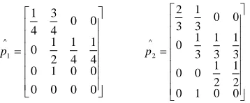
Based on the principle of the Markov chain model, the transition probability of the number of the interna-tional athletes and the number of the nainterna-tional athletes can be obtained:

                 0 0 0 0 0 0 1 0 4 1 4 1 2 1 0 0 0 4 3 4 1 ^ 1 p                    0 0 1 0 2 1 2 1 0 0 3 1 3 1 3 1 0 0 0 3 1 3 2 ^ 2 p

The result p1 p2 shows the transition probabilities

between various grades, so as to infer the next number of grade.

2.3.2 Grey model prediction

Here, this paper carries out prediction taking the number of international athletes who participate in the match as an example.

a. Grade ratio test

The times series to establish the number of athletes who participate in the match are as follows:

))

1

(

,

),

1

(

),

1

(

(

(0) (0) (0)

) 0 (

x

x

x

x





) 80 , 49 , 71 , 62 , 57 , 45 , 41 , 2 ( 

(1) Grade ratio



(

k

)

)

(

)

1

(

)

(

₍₀₎

) 0 (

k

x

k

x

k







(19)

))

7

(

,

),

3

(

),

2

(

(













)

6125

.

0

,

449

.

1

,

873

.

0

,

919

.

0

,

789

.

0

,

911

.

0

,

049

.

0

(



(20)

From (18), we know that the grade ratio is not within the accommodated coverage range

)

,

(

7 2

2 1 7 2   

e

e

. The conversion process of the series )

0 (

x

is to make it in the accommodated coverage range. Take the constant

c



200

for translation transformation:

n

k

k

x

k

y

(0)

(

)



(0)

(

)



200

,



1

,

2

,



,

(21) Then the grade ratio is:

) 96 . 0 , 92 . 0 , 08 . 1 , 94 . 0 , 05 . 1 , 19 . 1 ( 



(22)

(2) Grade ratio judgment

From (22), we know



(0.78,1.24), so (0)

(

)

k

y

can be used for

GM

(

1

,

1

)

model prediction. b.GM(1,1) Modeling

(1) Accumulate the original data (0)

y

:

)

407

,

327

,

278

,

207

,

145

,

88

,

43

,

2

(

) 1 (



y

(2) Construct the data matrix Band the data vector

Y:                                         ) 7 ( ) 3 ( ) 2 ( , 1 )) 7 ( ) 6 ( ( 2 1 1 )) 3 ( ) 2 ( ( 2 1 1 )) 2 ( ) 1 ( ( 2 1 ) 0 ( ) 0 ( ) 0 ( ) 1 ( ) 1 ( ) 1 ( ) 1 ( ) 1 ( ) 1 ( y y y Y y y y y y y B    (23) (3) Calculate ^

u

: ) 94 . 2 0017 . 0 ( ) ( ) , ( 1 ^      Y B B B b a

u T T T

(24)

Then

a





0

.

0017

,b2.94. (4) Modeling:

94

.

2

0017

.

0

(1)

) 1 (





y

dt

dy

(25)

(0) (0) (0) (0)

^ ^ ^ ^

( (1), (2), (7))

(43.5358,112.3976,192.4361, 322.5251, 350.1304, 426.6195, 507.3315)

y  y y y



The predicted value is an accumulated value, which is basically consistent with the original data which shows the rationality of the model.

3 PRINCIPLE OF ANALYTIC HIERARCHY

PROCESS (AHP) [6]

AHP can solve decision-making problems that are related to more complicated and ambiguous questions. Generally, the following four steps are required to constructing this model by the use of this method:

1. Establish the program of the hierarchical struc-ture;

2. Construct the matrix that is totally used for judgment at each level;

3. Test single hierarchical arrangement and con-sistency;

4. Test total hierarchical arrangement and con-sistency;

The model is designed to evaluate the Markov chain model and the grey prediction model. For the gymnas-tics trampoline training, which kind of data mining mode is more effective? The detail process of each step is respectively described below.

3.1 Hierarchical structure

The problems solved by AHP _{shall be hierarchical,}

methodical and logical. Only in this way can construct the hierarchical scheme. The elements in the compli-cated issues form multiple progressive levels accord-ing to their properties, degree of membership and the partnership. The elements of the last level can play a dominant role. In general, these levels are divided into three categories:

(1) Top level: This level contains only one factor. Generally, it is the ultimate goal of the issues re-searched, which can also be called as the target level. For this evaluation process, the target of the top level is a data mining mode suitable for gymnastics training. (2) Middle level: This level is an intermediate pro-cess involved in the achievement of targets. It may be multiple levels, containing multiple and multi-level criterion, which can also be called as the criterion level. The criterion level contains the simplicity of calculation, the rationality of results and the guiding significance of practical training.

(3) Bottom level: This level contains a variety of methods and means that are available for the achievement of the targets, which can also be called as the measure level or the scheme level. This evaluation compares with two data mining modes, including the

Markov chain prediction and the grey model predic-tion.

3.2 Construction of judgment matrix

The structure between each level is capable of show-ing the relationship between the factors, but the pro-portion of various factors of the middle level in the target evaluation is basically not the same. In the minds of evaluators, various factors have a certain proportion.

In determining the proportion of various factors, it is compared with the degree of impact of

n

factor(s)



1

,

,

n



X



x

x

on the factorZ.

Saaty

et al. pro-pose to compare the factors, and build a method of comparison matrix. That is to say, two factors

x

_i and

x

_j are selected at each time.

a

_ij is used to represent the proportion of the degree of impact of

i

x

and

x

_jon Z. All the comparison is expressed by the matrix

A



 

a

ij _{n n} .

A

becomes the judgment

matrix between

Z



X

. As can be seen from the matrix, if the proportion of the impact of

x

_iand

x

_jon Z is

a

_ij, then the proportion of the impact of

x

_j

and

x

_i on Z is ji 1 ij a

a

 _.

According to the theoretical knowledge of linear algebra, if the matrix

 

n n ij

a

A



_ satisfies

a

_ij



0

and



i

j

n



a

a

ij

ji

,

1

,

2

,

,

1







, then the matrix

A

is

the positive reciprocal matrix.

The matrix

A

is corresponding to the eigenvector

W

of the maximum value



_max of the characteristic value through normalization, that is, the corresponding elements in the same level are corresponding to the ordering weight value of some factors in the last level. This process is called as the single hierarchical ar-rangement and this process can reduce the interference of other factors, but there is inevitably inconsistency in the comprehensive comparison results. If the com-parison results are consistent, the factor

A

shall be met:

n

k

j

i

a

a

a

_{ij jk}



_ik

,



,

,



1

,

2

,



,

(26)

The positive reciprocal matrix satisfying the above formula is called as the consistent matrix. To deter-mine whether

A

can be accepted, there is a must to verify whether the inconsistency of

A

is very serious.

1.

A

must be a positive reciprocal matrix.

2. The transposed matrix ATis the consistent ma-trix.

3. Any two rows of the matrix of

A

are in propor-tion, and the factor is greater than 0, so rank

 

A 1, with the same row.

4. For _n

max

 in

A

,

n

is the order of the matrix

A

. Other characteristic root of the matrix

A

is 0.

5. The eigenvector W





T

n w w

W 1,, of



max,

then:







































n n n

n

n n

w

w

w

w

w

w

w

w

w

w

w

w

w

w

w

w

w

w

A















2 1

2

2 2

1 2

1

2 1

1 1

(27)

A

is the positive reciprocal matrix of

n

order(s). When it is the consistent matrix, if and only if

n



max



_{and when}

A

_{is inconsistent, then}

n



max



_{. Accordingly, the relationship between}

max

[image:6.516.54.251.132.286.2]



_and

n

_{can be used to verify whether}

A

_{is the} consistent matrix.

Table 4. Importance of influence factors of data mining modes.

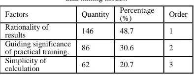
Factors Quantity Percentage _(%) Order Rationality of

results 146 48.7 1 Guiding significance

of practical training. 86 30.6 2 Simplicity of

calculation 62 20.7 3

The construction of the judgment matrix firstly needs to determine the importance of three factors in selection of data mining modes. In sports colleges and universities, the questionnaire survey is carried out based on these three influence factors, extracting the respondents (sports college students, sports coach and relevant personnel of sports) with the quota sampling [7]_{. 300 questionnaires are distributed in various} re-gions, including 281 valid questionnaires actually recovered, with the effective recovery rate of more

than 90%. The survey results are as shown in Table 4. Accordingly, the judgment matrix can be con-structed as follows:

According to the data in Table 4 and combined with the construction principle of the judgment matrix, the comparison matrix of the target level is constructed, which is shown in Table 5.

Table 5. Pairwise comparison matrix of the target level.

A B1 B2 B3

B1 1 3 5

B2 1/3 1 3

B3 1/5 1/3 1

The comparison matrix of the scheme level is to compare several schemes under an influence factor. The matrix construction method is the same with the above matrix construction method with an illustration.

1

P represents the grey model prediction, whileP2

[image:6.516.277.447.298.332.2]

represents the Markov chain model prediction.

Table 6. Pairwise comparison matrix (B1) of the scheme level.

B1 P1 P2

P1 1 3

P2 1/3 1

The above calculation process can be calculated through Matlabsoftware programming. The calcula-tion results are shown in Table 7.

As can be seen from Table 7, the grey model pre-diction is more suitable for the data mining of gym-nastics training. In terms of the calculation conven-ience, the Markov chain prediction method is more convenient. In case of a small amount of data, the Markov chain prediction is not accurate.

4 CONCLUSION

The Markov chain model requires to be supported by a large amount of data. For the practical problems in the inconvenience of data collection, the applicability of this model is not strong. The Markov chain model is established for the events with results that are free from the impact of historical results. Therefore, it is widely used in real life. The grey prediction method overcomes the difficulties in unpredictable variables of a single data. Due to its convenience and rapidness, it is also widely applied to various fields. For the data mining modes of gymnastics training due to a small

Table 7. Calculation results.

Target level B1 B2 B3

Total weight Weight of the target level 0.5543 0.3389 0.1068

[image:6.516.55.252.404.480.2]

amount of data, the grey prediction method is more appropriate.

REFERENCES

[1] Zhang Hongchen. 2014. Shanghai composite index forecasting by data mining in Sina Weibo, Master’s The-sis of Capital University of Economics and Business. [2] Liu Han. 2013. Research and application of China’s

macroeconomic mixing data model, Master’s Thesis of Jilin University.

[3] Xie Xiangyang. 2013. Research and application of data mining in sports data analysis, Contemporary Sports Technology, 3 (23): 9-10.

[4] Li Xuwen. 2010. Research on the development charac-teristics of China’s trampoline athletes, Master’s Thesis of Xi’an Physical Education University.

[5] Zhou Yongzheng, et al. 2010. Mathematical modeling. Shanghai: Tongji University Press.

[6] Wang Xiaoyin, et al. 2010. Mathematical modeling and mathematical experiment. Beijing: Science Press. [7] Wan Xinghuo. 2007. Probability and Mathematical