Modeling of Uncertainty in Dose Assessment using Probability Possibility Transformation

(1)

Modeling of Uncertainty in Dose Assessment using

Probability-Possibility Transformation

Tazid Ali

Dept. of Mathematics Dibrugarh University Dibrugarh-786004, India

Palash Dutta

Dept. of Mathematics Dibrugarh University, Dibrugarh-786004, India

ABSTRACT

Uncertainty parameters in risk assessment can be modeled by different ways viz. probability distribution, possibility distribution, belief measure, depending upon the nature and availability of the data. Different transformations exist for converting expression of one form of uncertainty to another form. In this paper, we reviewed the consistency principles as given by different researchers. Then we have carried out dose assessment using probability- possibility transformation satisfying consistency conditions.

KEYWORDS

Uncertainty, Risk Assessment, Probability-possibility transformation

1 INTRODUCTION

In some situations, some models parameters of radiological risk assessment may be affected by variability and uncertainty simultaneously. Basically, transforming probabilistic data to possibilistic data is useful when weak source of information make probabilistic data unrealistic. Also, it is useful in order to explore the advantages of possibilistic theory at combination steps, or perhaps to reduce the complexity of the solution when computing with possibility values rather than with probability values.

Transforming from possibility to probability may be meaningful in the case of decision making where a precise outcome is often preferred, such that, the decision maker is interested to know “what is likely to happen in future”, instead of “what is possible in future” [8].

According to [3] transforming possibility measure into probability measure or conversely can be useful in any problem where heterogeneous uncertain and imprecise data must be dealt with (e.g. subjective, linguistic like evaluation and statistical data).The possibilistic representation is weaker because it explicitly handles imprecision (i.e., incomplete knowledge) and because possibility measure are based on ordering structure rather than additive one. Therefore, it can be concluded that transforming a probabilistic representation to possibilistic representation, some information is lost because we go from point value probabilities to interval values ones. The converse transformation from possibility adds information to some possibilistic incomplete Knowledge.

Different transformations exist for converting expression of one form of uncertainty to another form. They differ from one another substantially, ranging from simple ratio scaling to more sophisticated transformation based upon various principles. These transformations should satisfy certain consistency principles. Here, we reviewed the consistency

principles as given by various authors viz., Zadeh, Klir, Dubois & Prade. Then dose assessment is carried out using Probability-Possibility transformations (as [1]).

2 TRANSFORMATION CONSISTENCY

PRINCIPLES

When information regarding some phenomenon is given in both probabilistic and possibilistic terms, the two descriptions should be in some sense consistent. That is, given

probabilistic representation

p

_iand possibilistic representation

i



on X, the two representations should satisfy some consistency condition. Although various consistency conditions may be required, the weakest one acceptable on intuitive groups can be expressed as follows:

An event that is probable to some degree must be possible at least to the same degree. That is, the weakest consistency condition is expressed formally by the inequality

i i

p





On the other hand, the strongest consistency condition would require that any event with nonzero probability must be fully possible.

0

1.

i i

p

 





In this section different consistency principles [2], [5], [7], [10] are reviewed

2.1. Zadeh consistency principle

Zadeh defined the probability-possibility consistency principle such as “a high degree of possibility does not imply a high degree of probability, nor does a low degree of probability imply a low degree of possibility” (Zadeh 1978).

Let U be a finite set. X is a variable taking a value in U.



_i

and

p

_iare possibility and probability that X = ui ϵ U

respectively. Then, Zadeh’s consistency principle can be expressed by

0

i

p

i



 



and



_i>



_j



p

_i



p

_j. He defined the degree of consistency between a probability

and a possibility distribution

(2)

1

...(1)

n

i i i

r



p





From (1), it can be check that

(i) if



_i

 

0,

i

then

r



0

, no consistency available. An impossible event cannot be probable.

(ii) If



_i

 

1,

i

then

r



1

, the maximum consistency value is reached. Any probability measure is still consistent with this probability measure.

Maximizing the degree of consistency, however, poses us a

very restrictive condition that;



_i

 

1 p

_i



0. 2.2: Klir consistency principle:

Let

X



{ ,

w w

₁ ₂

,....

w

_n

}

be a finite universe, let

(

)

i i i

p



p w

and



_i





_i

(

w

_i

)

. Assume that the elements of

X

are ordered in such a way that:

1

1, 2,... :

_i

0,

_i _i

i

n p

p

_

 





and

1

0,

i i i





 



_ with

p

n1



0

and



n1



0

.

According to Klir the transformation from

p

_i to



_i must preserve some appropriate scale and the amount of information contained in each distribution (Klir 1993).The information contained in

p

or



can be expressed by the equality of their uncertainties. Klir has considered the principle of uncertainty preservation under two scales.

The ratio scale: This is a normalization of the probability distribution. The transformation

p





and

p





are named the normalized transformations and they are defined by

1

,

...(2)

i i

i i n

i i

p

n







The log-interval scales: the corresponding transformation

p





and





p

are define by:

1

1 1

1

(

i

) ,

i

...(3)

i i _n

i i

p

 









These transformations are known as Klir transformation satisfying the uncertainty preservation principle defined by Klir (1993).



is a parameter that belongs to the open interval (0, 1). According to Klir any transformation should be based on the following three assumptions:

- A scaling assumption that forces each value (



_i) i to be a

function of pi/p1 (where p1≥p2≥……≥pn) that can be ratio scale,

interval scale, log-interval scale transformation etc.

- An uncertainty invariance assumption according to which the entropy H(p) should be numerical equal to the measure of information E(



_i) contained in the transformation



_i to p. - The transformation should satisfy the consistency condition





(u) ≥ p(u),



i, starting that what is probable must be possible.

Dubois and Prade gave an example to show that the scaling assumption of Klir may some time lead to violation of the consistency principle that requires  Pfor all events. The second assumption is also debatable because it assumes possibilistic and probabilistic information measures are commensurate.

5.2.3: Dubois and Prade consistency

Principle

The transformation

p





is guided by the principle of maximum specificity, which aims at finding the most informative possibility distribution. While the transformation

p





is guided by the principle of insufficient reason which aims at finding the possibility distribution that contains as much as uncertainty as possible but that retains the features of possibility distribution (Dubois 1993). This leads to write the consistency principle of Dubois and Prade such as:

:

( )

( )...(4)

A

X



A

p A

 



The transformation

p





and





p

are define by

1

(

)

;

...(5)

n n

j j i j i

j i j i

p

j





 











The two transformations define by (5) are not converse of each other because they are not based on same informational principle. Therefore, the transformation defined by (5) can be named as asymmetric. Dubois and Prade suggested a symmetric

p





transformation which is define by:

min(

,

)...(6)

n

i i j

j i

u

p p





Dubois and Prade proved that the symmetric transformation

p





, define by (6), is the most specific transformation which satisfies the condition of consistency of Dubois and Prade define by (4).

5.3 Probability

to

Possibility

Transformation

Transforming probabilistic data to possibilistic data is useful when weak source of information make probabilistic data unrealistic. Also, it is useful in order to explore the advantages of possibilistic theory at combination steps, or perhaps to reduce the complexity of the solution when computing with possibility values rather than with probability values [8].

5.3.1 Normal

probability

distribution

function to Gaussian fuzzy number

(3)

or Trapezoidal shape fuzzy numbers some other types of fuzzy numbers come into picture viz., Gaussian fuzzy number, lognormal shaped fuzzy number etc.

To define a fuzzy number in the form of Gaussian distribution and so, the membership function required for building the Gaussian shaped fuzzy set must be expressed as follows [9]:

2

1 (

)

( )

exp

2

2 x

f x





 



 





_

_





where



and



represent the mean and the standard deviation respectively.

By definition, a fuzzy number is a fuzzy set whose

membership function

:

[0,1]

:

( ) 1

A

R

x

R

A

x





 





i.e., there must

be at least one domain element whose membership grade equals 1, and normal.

Hence, by normalizing the fuzzy set, we obtain the following expression for membership function of the fuzzy set (Pacheco et al, 2009):

2

(

)

( ) exp

...(7)

2

A

x







 





_

_





For fuzzy set to become convex, one calculates the inflexion points of the domain of the Gaussian by making the second

derivative equal to zero, i.e.,

f

''

( ) 0

x



. Thus, the domain of the normalized and convex fuzzy set is formed by the interval

[

   



,



].

However, for this domain, only 68% of the information contained in the Gaussian will be represented by the fuzzy number. Due to small amount of Gaussian information contained in the fuzzy set, we consider considered a new interval,

[





3 ,

 



3 ]



, as the domain of the fuzzy number which represents approximately 99.7% of the information contained in the Gaussian and established an



-cut at 0.01. Here, convexity constrained is relaxed and operation on Gaussian fuzzy number is performed.

The domain R of the fuzzy number is bounded to the interval

[





3 ,

 



3 ]



and whose



-cut is placed at 0.01.

For this fuzzy number, the



-cut is defined as:

[

2ln ,

2ln

]

A



_

_{ }

_

_{  }

_

_

_

Where



and



represent the mean and the standard deviation respectively and



corresponds to the



-cut defined in the interval [0.01, 1]. Then interval arithmetic can be applied to perform operations on Gaussian fuzzy numbers, where each possibilistic interval defined by the



-cut can be treated independently.

5.3.2 Triangular probability distribution

function to triangular fuzzy number

A random variable X is said to be triangularly distributed with lower limit a, upper limit c and mode b such that , the probability density function is given by





















otherwisw

c

x

b

a

b

c

x

c

b

x

a

c

a

b

a

x

f

,

0 ,

)

)(

(

)

(

2 ,

)

)(

(

)

(

2 )

(

Normalizing the distribution function (dividing the function by the maximum height i.e., by 2/(c-a)) we will have the fuzzy number whose membership function is

,

A

x

a

x

b

a

c

x

b

x

c

b







_{ }

 

 

_



_{ }

 



5.4 Possibility

to

Probability

Transformation

Transforming from possibility to probability may be meaningful in the case of decision making where a precise outcome is often preferred, such that, the decision maker is interested to know “what is likely to happen in future”, instead of “what is possible in future” [8].

5.4.1 Gaussian fuzzy number to normal

probability distribution function

As authors in [9] defined the Gaussian fuzzy number, whose membership function is

2

(

)

( ) exp

2

A

x







 





_

_





where



and



Whenever we have mean and the standard deviation and the shape of the distribution, so in such situation where a precise outcome is often preferred, we can consider its probabilistic form as follows:

2

1 (

)

( )

exp

2

2 x

f x





 



 





_

_





where



and



5.4.2 Triangular

fuzzy

number

to

triangular probability distribution function

Consider a triangular fuzzy number A= [a, b, c] whose membership function is given as:

,

A

x

a

x

b

a

c

x

b

x

c

(4)

Integrating the Fuzzy set with respect to x on [a, c] we have,

c b c

A A A

a a b

dx













1

1 (

)

(

)

b c

a b

x

a dx

c

x dx

b

a

c

b















2 2

1

2

b c

a b

x

ax

cx

b

a

c

b











_



_



_



_



_

_



_

_

2 2 2 2

2 2

1

2

2 b

a

c

b

ab

a

c

bc

b a

c b











_





_



_



 

_



_

_



_

_

2 2 2 2

1

1 (

)

(

)

(

)

(

)

2 b

a

a b a

2 b

c

c b c

b a

c b











_



_



_



_













1 1 1 1

( ) ( ) ( ) ( )

2 2

b a b a a c b b c c

b a c b

   

  _   _  _   _

     

1 1

( ) ( )

2 2

1

( )

2

b a b c

c a

   

 

Dividing the Fuzzy set (8) by

1 (

)

2 c



a

, we get

the probability distribution function

2(

)

,

[image:4.595.323.532.278.443.2] [image:4.595.332.521.495.634.2]

(

)(

)

( | , , )

2(

)

,

(

)(

)

x a

a

x

b

b a c a

f x a b c

c

x

b

x

c

c b c a





_{ }

 





 

_



_{ }

 





5 DOSE

ASSESSMENT

USING

PROBABILITY-POSSIBILITY

TRANSFORMATION

5.1 Problem definition

Here, we have considered a case of soil contamination by lead on an ironworks Brownfield in the south of France. Following an on-site investigation revealing the presence of lead in the superficial soil at levels on the order of tens of grams per kg of dry soil, a cleanup objective of 300 mg/kg was established by a consulting company, based on a potential risk assessment, taking into account the most significant exposure pathway and the most sensitive target (direct soil ingestion by children).

5.2 Dose Assessment Model

The mathematical model calculating the quantity Dlead

absorbed by a child living on the site and exposed via soil ingestion is given by EPA, (1989) [6].

6

(

)

...(9)

10

soil soil inside outside lead

C

IR

Fi

EF ED

D

Bw AT











where, Dlead is the absorbed lead dose related to the ingestion

of soil (mg/[kg:day]), Csoil is the lead concentration in Soil

(mg/kg),IRsoil is the ingestion Rate mg soil/day, Fiindoor is the

indoor Fraction of contaminated soil ingestion (unitless), Fioutdoor is the outdoor Fraction of contaminated soil ingestion

(unitless), E F is the exposure Frequency (days/year), EDis the exposure Duration (years), Bw is the body Weight (kg), AT is the Averaging time (period over which exposure is averaged–days)

5.3 Results and discussion

Here, we have considered three scenarios. In scenario1, representations of some model parameters are probabilistic while some are probabilistic. In scenario2, possibilistic model parameters are transformed into probabilistic mode while in scenario3, probabilistic model parameters are transformed into possibilistic mode.

5.3.1 Scenario1

Here, representations of the parameters Csoil as well as Fiindoor

are possibilistic and IRsoil and Bw are probabilistic and other

parameters are deterministic.

Table 1 Parameter values used in the dose assessment

Variable Mode of

Representation Value

Csoil Fuzzy TFN(40,300,500)

IRsoil Probabilistic Triangular(20,160,300)

Fiindoor Fuzzy TFN(0.2,0.55,0.9)

Fioutdoor Deterministic 1.0

EF Deterministic 273.75 ED Deterministic 6

AT Deterministic 6×365 = 2190 Bw Probabilistic Normal(17.2,2.57)

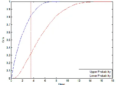
The graphical representation of the result of the calculation using hybrid method [4] is given in figure 1.

Fig. 1: Plot of upper and lower probability function for estimating dose

According to the World Health Organization prescribed the acceptable lead dose related to the ingestion of polluted soil to be equal to 3.5 µg/[kg:day]. That means that after the cleanup objective of 300 mg/kg on the site (ironworks Brownfield), calculated doses Dlead should not be larger than 3.5

(5)

imprecision regarding input parameters leads to a clearer rejection of the proposition Dlead < 3.5 µg/[kg:day]. The gap

between the lower probability and upper probability reflects the imprecision of some model parameters.

5.3.2 Scenario2

[image:5.595.322.533.87.251.2]

In this scenario, possibilistic model parameters are transformed to probabilistic mode (section 4). Parameter values used in this calculation are given in the following table 2.

Table 2: Parameter values used in the dose assessment

Variable Mode of

Csoil Probabilistic Triangular(40,300,500)

IRsoil Probabilistic Triangular(20,160,300)

Fiindoor Probabilistic Triangular(0.2,0.55,0.9)

AT Deterministic 6×365 = 2190 Bw Probabilistic Normal(17.2,2.57)

The graphical representation of the result of the calculation using proposed method (previous chapter) of scenario 2 is given in figure 2.

Fig. 2: Plot of probability function for estimating dose

Here, we have seen from the figure 2 that probability of dose value less than 3.5 µg/[kg:day], is 0.576 which is not enough to consider to be a low dose i.e., to accept the proposition Dlead < 3.5 µg/[kg:day].

5.3.3 Scenario3

[image:5.595.59.275.200.366.2]

In this scenario, probabilistic model parameters are transformed to possibilistic mode (section 3). Representation the parameter body weight (Bw) is a Gaussian fuzzy number with mean 17.2 and standard deviation is 2.57. Parameter values used in this calculation are given in the following table 3.

Table 3: Parameter values used in the dose assessment

Variable Mode of

Csoil Fuzzy Triangular(40,300,500)

IRsoil Fuzzy Triangular(20,160,300)

Fiindoor Fuzzy Triangular(0.2,0.55,0.9)

AT Deterministic 6×365 = 2190 Bw Fuzzy Gaussian(17.2,2.57)

Here, we will relax the convexity condition to combine Gaussian fuzzy number and triangular fuzzy number using



-cut by considering that



corresponds to the



-cut defined in the interval [0.01, 1]. It will not affect the uncertainty involved in the fuzzy number.

The result of the dose assessment of scenario 3 is depicted in figure 3.

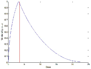
Fig. 3: Plot of membership function for estimating dose

The resulting dose is also obtained in the form of a fuzzy number as some input parameters are available in the form of fuzzy number. 3.244 is the core of the output fuzzy dose while the range is [0.03292, 22.5]. Here, the threshold value 3.5 µg/[kg:day] slightly exceeds the core value with membership value 0.976 and it belongs to the range [0.03292, 22.5]. Here, also consideration of imprecision regarding input parameters leads to a clearer rejection of the proposition Dlead < 3.5

µg/[kg:day].

6. CONCLUSION

[image:5.595.330.524.361.507.2] [image:5.595.69.264.428.570.2]

(6)

probability-possibility transformations arises not only from a desire to comprehend the relationship between the two theories of uncertainty, but also for some practical problems. For example: to construct a membership grade function of a fuzzy set from statistical data, to construct a probability measure from a given possibility measure in the context of decision making or system modeling, to combine probabilistic and possibilistic information in expert systems, or to transform probabilities to possibilities to reduce computational complexity. To deal with these problems, various probability-possibility transformations satisfying different consistency principles have been suggested in the literature. Here, we have considered a case of soil contamination by lead on an ironworks Brownfield in the south of France. Following an on-site investigation revealing the presence of lead in the superficial soil at levels on the order of tens of grams per kg of dry soil, a cleanup objective of 300 mg/kg was established by a consulting company, based on a potential risk assessment, taking into account the most significant exposure pathway and the most sensitive target (direct soil ingestion by children). The assessment is carried out by considering there scenarios. In scenario1, representations of some model parameters are probabilistic while some are probabilistic. In scenario2, possibilistic model parameters are transformed into probabilistic mode while in scenario3, probabilistic model parameters are transformed into possibilistic mode. In each scenario, we have seen the clear rejection of the World Health Organization prescribed the acceptable lead dose related to the ingestion of polluted soil to be equal to 3.5 µg/[kg:day].

ACKNOWLEDGEMENT:

The work done in this paper is under a research project funded by Board of Research in Nuclear Sciences, Department of Atomic Energy, Govt. of India.

REFERENCES

[1] Ali T., Dutta P., Boruah H., (2011), Comparison of a Case Study of Uncertainty Propagation using Possibility - Probability Transformation, International Journal of Computer application, 35:47-55.

[2] Dubois D., Prade H., Sandri S. (1993): On possibility/ probability transformations, in Fuzzy Logic: State of the Art,R. Lowen and M. Lowen, Eds. Boston, MA: Kluwer,pp. 103-112.

[3] Dubois D., Foulloy L., Mauris G., Prade H. ( 2004): Probability-Possibility Transformation, Triangular Fuzzy Sets and Probabilistic Inequalities, in ReliableComput., 10:273-297

[4] Dutta P., Ali T., (2012), A Hybrid Method to deal with aleatory and epistemic uncertainty in risk assessment, International Journal of Computer Applications, 42 :37-44.

[5] Elena Castineira, Susana Cubillo, Enric Trillas (2007): On the Coherence between Probability and Possibility Measures, International Journal “Information & Applications” 14:303-310.

[6]. EPA, U.S. (1989) Risk Assessment Guidance for Superfund. Volume I: Human Health Evaluation Manual (Part A). (EPA/540/1-89/002).O_ce of Emergency and Remedial Response. U.S EPA., Washington D.C.

[7] Mouchaweh M.S., Bouguelid M.S., Billaudel P., Riera B. (2006): Variable Probability-possibility Transformation, 25th European Annual Conference on Human Decision-Making and Manual Control (EAM'06), September 27-29, Valenciennes, France.

[8] Oussalah, M. (2000): On the probability /possibility transformations: a comparative analysis, Int. journal of General system, 29:671-718

[9] Pacheco M. A.C., Vellasco M .B. R. (2009): Intelligent Systems in Oil Field Development under Uncertainty. (Springer-Verlag, Berlin Heidelberg.)