Neuro-Wavelet based Efficient Image Compression
using Vector Quantization
Arun Vikas Singh
Research Scholar,VTU, Belgaum, Department of ECE, PESIT, Bangalore,
Karnataka, India
Srikanta Murthy K
Professor and Head Department of CSE, PESSE,
Bangalore, Karnataka, India
ABSTRACT
In the last few decades, Digital image compression has received significant attention of researchers. Recently, based on wavelets there has been many compression algorithms. In comparison to other compression techniques, image compression using wavelet based algorithms lead to high compression ratios. In this paper, we have proposed a image compression algorithm which combines the feature of both wavelet transform and Radial Basis Function Neural Network along with vector quantization. First the images are decomposed into a set of subbands having different resolution with respect to different frequency bands using wavelet filters. Based on their statistical properties, different coding and quantization techniques are employed. The Differential Pulse Code Modulation (DPCM) is used to compress the low frequency band coefficients and Radial Basis Function Neural Network (RBFNN) is used to compress the high frequency band coefficients. The hidden layer coefficients of RBFNN subsequently are vector quantized so that without much degradation of the reconstructed image, the compression ratio can be increased. In terms of peak signal to noise ratio (PSNR) and computation time (CT), a large compression ratio has been achieved with satisfactory reconstructed images in relation to the existing methods by using the proposed technique.
Keywords
Image Compression, Radial Basis Function Neural Network, Back-Propagation Neural Network, Vector Quantization.
1.
INTRODUCTION
In the field of mobile and video communication, image compression is one of the enabling technologies. The image has to be encoded into fewer bits in order to reduce the storage requirements in image archival systems, or to reduce the bandwidth for image transmission. Moreover, image compression plays a very important role in many major and diverse applications, like document and medical imaging, remote sensing, televideo conferencing, facsimile transmission and the control of remotely piloted vehicles in space, military and in hazardous waste management.
In data compression and coding, the use of sub band decomposition has been extensively used [1]. Crochiere et al. [2] was the first to propose sub band coding for medium bandwidth waveform coding of speech signals. The extension of sub band decomposition to two-dimensional (2-D) signals was demonstrated by Woods and O‟Neil [3]. The possible aliasing error due to non ideal sub band filters were removed by proposing a method for Quadrature mirror filters (QMF) design. The current progress in the field of signal processing tools for instance wavelets, has opened a new horizon in sub
band image coding. The recent study in wavelet transform reveals that it exhibits the frequency selectivity as well as orientation of images [4]. The wavelet bases represent a large class of signals, thereby enabling us to notice roughly isotropic features occurring at all spatial scales and locations. Due to these reasons wavelets are more successful. The image is decomposed using different wavelet filters and encoded using SPIHT as proposed in [5] for image compression. For image compression, the computation in Haar and Fast Haar wavelet transforms is reduced by using the modified fast Haar wavelet transform [6].
The inherent parallel processing capabilities of neural network based approaches [7] used for data processing, have yielded very promising results. The training scheme permits the network to be suitable for diverse data. Sonhera et. al propose a technique [8] where the number of units (neurons) in input and output layers remains the same in a two layered neural network and has reduced the number of units (neurons) in hidden layers. Using Kohonen Self-organizing Features Map (SOFM) Gersho et al [9] have designed a codebook for vector quantization of images. For multistage image compression, Hussan et.al [10] have proposed a dynamically constructed neural architecture where for a given image compression quality, the necessary number of hidden layers and the number of units in each hidden layer are determined automatically.
A neuro-wavelet based approach for image compression using fuzzy vector quantization has been presented by Vipula Singh et al [11] which combine the advantages of wavelet transform, neural network and fuzzy vector quantization. Chi-Sing Leung et al [12] have proposed an RBF-based compression method for image-based relighting where a two level compression method is presented. the plenoptic property of a pixel is approximated In the first level by a spherical radial basis function (SRBF) network . Then in the second level, a wavelet-based method is applied to compress these SRBF weights. Adnan khashman et al [13] have proposed a technique for image compression using neural networks and haar wavelet where authors claims that after presenting the image to the network, a back-propagation neural network (BPNN) could be trained to recognize an optimum ratio for haar wavelet compression of an image
.
problems with non-stationary inputs because of the behavior of the radial basis function hidden units. Furthermore, the wavelet based decomposition dramatically improves the quality of reconstructed images as compared to the neural network based compression. Image compression using Discrete Cosine Transform (DCT) produces blocking effects in the reconstructed image. These blocking effects associated with DCT are eliminated by using wavelet decomposition. First the images are decomposed into a set of subbands having different resolution with respect to different frequency bands using wavelet filters. Based on their statistical properties, different coding and quantization techniques are employed. Differential Pulse Code Modulation (DPCM) is used to compress the low frequency band coefficients and Radial Basis Function Neural Network (RBFNN) is used to compress the high frequency band coefficients. The hidden layer coefficients of RBFNN subsequently are vector quantized so that without much degradation of the reconstructed image, the compression ratio can be increased. The conventional Back Propagation Neural Network (BPNN) with wavelets has been applied to the image set and a comparative study of this scheme with the RBFNN with wavelets has been carried out. The paper is organized as follows: Section 2 presents the brief theory of discrete wavelet transform. Section 3 discusses about multilayered neural network for image compression. Section 4 briefly presents Radial Basis Function Neural Network for image compression. Section 5 briefly presents the k-mean algorithm for vector quantization. Section 6 presents the proposed method for efficient image compression. Section 7 reports experimental results and section 8 provides concluding remarks.
2.
DISCRETE WAVELET TRANSFORM
For image compression, wavelets have recently emerged as a powerful tool. Image is mapped into a set of coefficients by using discrete wavelet Transform that constitutes a multiscale representation of the image [14]. By passing x(n) through a series of filters, Discrete Wavelet Transform (DWT) is computed. The approximation coefficients are generated by passing the samples through a low pass filter with impulse response g(n). Simultaneously, the signal is decomposed to give the detailed coefficients by using high pass filter h(n) as shown in Fig.1. The approximation coefficients are obtained at the output of low pass filter. These filters are known as quadrature mirror filters (QMF). The filter outputs are down sampled by 2 because half the frequencies of the signal are removed [14][15].
yhigh[k] = 𝑥 𝑛 . 𝑔[2𝑘 − 𝑛]𝑛 - low pass filter output ylow[k] = 𝑥 𝑛 . ℎ[2𝑘 − 𝑛]𝑛 - high pass filter output
Fig 1: One level Decomposition
Let x(m,n) represent an image which is a 2 dimensional signal. First each row is filtered and then two (m, n/2) images are obtained by down sampling it. Then each column is filtered and four (m/2, n/2)images are obtained by down
are obtained. The following functions are required for the image (two dimensions):
(i) One 2-dimensional scaling function 𝜑(𝑥, 𝑦) (ii) Three two-dimensional wavelet functions
𝛹H
(x,y), 𝛹V(x,y), 𝛹D(x,y)
[image:2.595.358.500.218.340.2]Further the approximation coefficients belonging to subband LL are then decomposed into four at level two. For the further levels the process can be continued in the same manner. Energy concentration is more in LL band as compared to other bands.
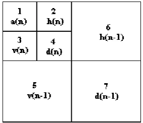
Fig 2: Two stages of pyramidal decomposition leading to 7 octave subbands
A three level wavelet decomposition scheme is shown in Fig. 2 for a 256*256 digital image. This decomposition method produces three side bands corresponding to resolution level1 having size 128*128. Further, it produces three side bands corresponding to resolution level 2 having size 64*64. The lowest frequency components of the original image lie in sub band image 1 and they have more energy as compared to other sub band images. The sub band images from 2 to 7 have detailed coefficients of edges. Sub band images 3 and 5 represent the vertical edge coefficients of image after first and second levels of wavelet decomposition respectively. Sub band images 2 and 6 represent the horizontal edge coefficients of image after first and second levels of wavelet decomposition respectively. Sub band images 4 and 7 represent the diagonal edge coefficients of the image after first and second levels of wavelet decomposition respectively. In this paper, the sub band image 1 is coded with DPCM and the remaining coefficients in sub band 2 to sub band 6 are compressed by neural network. The coefficients present in sub band 7 are discarded as it has less energy than the other sub bands.
3.
NEURAL NETWORK FOR DATA
COMPRESSION
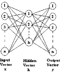
Image compression coding is one of the applications where Back-propagation neural network can be applied directly. Fig. 3 shows the multi layered neural network structure. Here three layered Back-propagation neural network is designed which consists of one input layer, one output layer and one hidden layer.
connected to all weights and can be described by {wij , j = 1,2, ... k and i = 1,2….... n}, which can also be represented in matrix form of size k x n.
The connections from the hidden layer to the output layer are represented by {wij}, is the weight matrix of size n x k, which is set equal to the transposition of matrix [w]. To achieve image compression, the network is trained in such a way that the weights wij scales the n dimensional input vector into a vector of k-dimension (k< n) at the hidden layer. Thus the optimum output value is produced which makes the quadratic error minimum between input and output layer.
Fig 3: A Multi Layered Neural Network
Let wij denote the weight from xi to hj, then n elements of input vector x are related to the k elements of hidden vector h by expression [11],
ni i ij
j
w
x
h
1j=1, 2, ……k (1)
The n elements of output vector y are given by the expression [11],
kj j ij
i
w
h
y
1
i=1, 2, ……n (2)
where, wij is the weight between hj and yi.
In order to minimize the distortion between the input vector and output vector, the weights of neural network are chosen. The squared error between input vector and output vector for the training set is minimized using back propagation algorithm. The normalized values of the wavelet coefficients are denoted by
x
[
1
,
1
]
. The compression is achieved using back propagation neural network in two phases. The first phase is the training phase and second phase is the encoding phase. In the training phase, using back propagation learning rule, a set of image samples is designed to train the network where each input vector is chosen as the desired output. Here, the input layer is compressed into the narrow channel which is represented by hidden layers and then the input is reconstructed from the hidden layer to the output layer. In the encoding phase, the compressed output is available at the hidden layer when the input is presented to the input layer.4.
RADIAL BASIS FUNCTION NEURAL
NETWORK FOR IMAGE
COMPRESSION
Supervised training algorithms are used to train Radial basis function networks which are feed-forward networks. The output function of Radial basis function networks is selected from a class of functions called basis functions which are configured with a single hidden layer of units. Fig.4 shows the basic structure of a Radial basis function networks which involves three different layers. The input layer consists of source nodes (sensory units) having dimension N which is equal to the input vector u. The second layer contains nonlinear units that are directly connected to all of the nodes in the input layer. This layer is called the hidden layer of Radial basis function network. The input from all the nodes at the components of the input layer is given to each corresponding hidden unit. Each hidden units contains a basis function having the parameters, center and width. The vector ci, represents the center of the basis function for a node i at the hidden layer. The size of the vector ci, is as that of the input vector u. Similarly, each unit in the network has a different center.
The radial distance di, is the difference of the the input vector u and the center of the basis function ci. This radial distance is calculated for each unit i in the hidden layer and is given by
[image:3.595.78.215.205.368.2]the Euclidean distance, di = │u – ci │ (3)
Fig 4: Structure of the standard Radial Basis Function Network
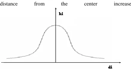
By applying the basis function G to the radial distance di, the output hi is computed for each hidden unit i, given by
distance from the center increases.
Fig 5: The response region of an RBF hidden node around its center as a function of the distance from this center.
5.
QUANTIZATION
The amount of the data is not reduced by applying the wavelet transform on images. The number of bits required for the compression phase can be reduced by quantizing the coefficients and then applying lossless compression techniques such as arithmetic or Huffman coding to the quantized coefficients.
5.1
Vector Quantization (VQ)
A vector quantizer Q having dimension n and size k is represented as a mapping from a vector that lie with in a region in n-dimensional Euclidean space Rn, into a set y which is finite containing k vectors. These k vectors are called codebook vectors or codewords. The mapping can be represented as Q: Rn→ y , where Y = {y1,y2,…...,yk}, and yi∈ R
n∀
j=1,2,...,k. The set y represents the codebook which has the size k. To design a vector quantizer, a set of training vectors are required which are called the training set. A training set is represented by set X having dimension n and size M is formed by M training vectors from an n- dimensional Euclidean space which is represented as X = {x1, x2, . . . , xM }, and xi ∈ Rn ∀ i=1,2,...,M. In vector
quantization, the M training vectors is assigned to k clusters and each cluster is represented by a codebook vector. This can be attained by minimizing the measure of the discrepancy between the codebook vectors and the training vectors. The codebook quality depends on the following criteria.
(i)The technique used for assigning training vectors to cluster. (ii)The strategy employed to minimize the discrepancy measure. (iii) The optimization technique employed to perform minimization of discrepancy measure.
The codebook design quality is measured frequently using average distortion and is defined as follows [11],
M i j i Y j y M ii
d
x
y
x
d
M
D
1 1min
(
)
min
(
,
)
1
(5)
5.1.1
k-Means Algorithm
On the basis of the nearest neighbor condition, the k-means algorithm assigns each training vector to a certain cluster. In accordance with this condition, the training vector xi is
assigned to the jth cluster if
)
,
(
min
)
(
)
,
(
x
iy
jd
minx
i yj yd
x
iy
jd
whered(xi, yj)is defined as the squared Euclidean distance between
the codebook vector yj and the training vector xi.
Mathematically d(xi,yj) can be represented as [11], 2
)
,
(
)
,
(
x
iy
jd
x
iy
jd
The nearest neighbor condition can be easily represented by a membership function, or selector function, which is stated as [11] otherwise x d y x d if x
uj i i j i
0 ) ( ) , ( 1 )
( min (6)
By minimizing a distortion measure, the codebook vectors are evaluated and is defined as [11],
2
1 1
1
( ) k j M i j i i
j x x y u
J (7)
The minimization of J1 = J1 (yj, j= 1 , 2 , . . k ) with respect to yjfor a given set of membership functions results in [11],
(8) Eqn. (8) defines the codebook vector yj and is the centroid or
Euclidean center of gravity of all the training vectors assigned to the jth cluster.
6.
PROPOSED METHOD
The image is first decomposed into 7 sub bands using wavelet transform. The following scheme is adapted since human visual system has different sensitivity for different frequency components. The DPCM encodes the lowest frequency band coefficients in sub band 1. These coefficients are further scalar quantized. The neural network (RBFNN/BPNN) is used to compress the remaining frequency band coefficients. For different orientations, band-2 and 3 contain the same frequency contents. Hence, in order to compress the data same neural network is used. For band-2 and 3 the neural network used have 16 units in input and output layer, and 12 units in hidden layer (16-12-16 neural network). Similarly, the same neural network (16-1-16) is used to compress the coefficients in band- 5 and 6 as it has same frequency contents for different orientations. Since the frequency characteristic of band-4 does not match with other bands, the coefficients of this band are compressed by a separate neural network (16-8-16). Since the coefficients in band-7 contain little information to contribute to the image, these coefficients are discarded, as the quality of reconstructed image is not significantly affected. The coefficients obtained at the output of the hidden layer of neural network are then vector quantized. In different sets of experiments the vector quantizer is used. Huffman encoding is used to encode these coefficients. Originally this scheme is proposed in [16].
7.
EXPERIMENTAL RESULTS AND
DISCUSSION
less susceptible to problems with non-stationary inputs because of the behavior of the radial basis function hidden units. Experiments were conducted using the gray scale images „lena‟, ‟girl‟, „girl(tiffany)‟, „pepper‟, „house‟ and „saturn‟ of size 256 x 256. The PSNR values obtained for Standard images by applying, the proposed technique using Wavelet transform with both RBFNN and BPNN algorithms are illustrated in Table 1. It is found from Table 1, that for a given bits per pixel (bpp), the proposed technique using Wavelet transform with RBFNN technique yields better PSNR and computation time (CT) is lesser than compared to Wavelet transform with BPNN. This is because RBFNN are usually trained much faster than back propagation networks. They are less susceptible to problems with non-stationary inputs because of the behavior of the radial basis function hidden units. Table 2 shows the PSNR and Computation Time (CT) of training image „lena‟ using vector quantization with
different wavelet filters. It is demonstrated from Table 2 that for different wavelet filters and given bits per pixel (bpp), the proposed technique using Wavelet transform with RBFNN technique yields better PSNR and takes less computation time (CT) than compared to Wavelet transform with BPNN. The PSNR and bpp of the reconstructed images („lena‟, ‟girl‟, „girl(tiffany)‟, „pepper‟, „house‟ and „saturn‟) for the proposed technique using Wavelet Transform with RBFNN and Wavelet Transform with BPNN approach is shown in Fig.6 to Fig.11. The reconstructed images with Wavelet Transform and BPNN are shown in Fig.12. The reconstructed images with the proposed technique using Wavelet Transform and RBFNN are shown in Fig.13. From the reconstructed images we can observe that the ringing effects are clearly visible in wavelet with BPNN technique. But by using the proposed wavelet with RBFNN technique this ringing affect has been eliminated in the reconstructed images. .
Table 1. PSNR of different test images reconstructed by db18 and vector quantization
Fig 6: (a) original (b) Reconstructed with BPNN &VQ (c) Reconstructed with RBFNN &VQ (PSNR is 25.9590 and bpp is 0.3934) (PSNR is 26.4717 and bpp is 0.3934)
Fig 7: (a) original (b) Reconstructed with BPNN &VQ (c) Reconstructed with RBFNN &VQ (PSNR is 28.5008 and bpp is 0.4269) (PSNR is 28.8224 and bpp is 0.4269)
Fig 8: (a) original (b) Reconstructed with BPNN &VQ (c) Reconstructed with RBFNN &VQ Image
With BPNN With RBFNN
PSNR bpp C T in seconds PSNR bpp CT in seconds
Lena 25.9590 0.3934 8.397995 26.4717 0.3934 7.533728
Girl 28.5008 0.4269 9.163019 28.8224 0.4269 7.390822
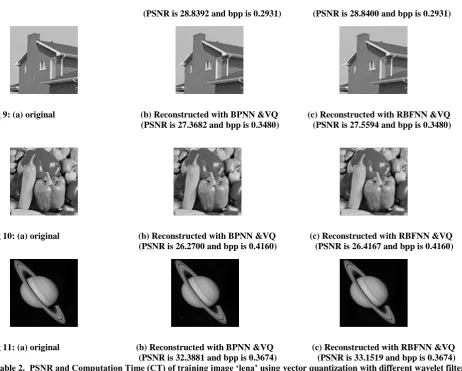
Girl (tiffany) 28.8392 0.2931 7.982073 28.8400 0.2931 7.360766
House 27.3682 0.3480 8.912658 27.5594 0.3480 7.505699
Peppers 26.2700 0.4160 8.897010 26.4167 0.4160 7.357871
[image:5.595.55.535.279.758.2](PSNR is 28.8392 and bpp is 0.2931) (PSNR is 28.8400 and bpp is 0.2931)
Fig 9: (a) original (b) Reconstructed with BPNN &VQ (c) Reconstructed with RBFNN &VQ (PSNR is 27.3682 and bpp is 0.3480) (PSNR is 27.5594 and bpp is 0.3480)
Fig 10: (a) original (b) Reconstructed with BPNN &VQ (c) Reconstructed with RBFNN &VQ (PSNR is 26.2700 and bpp is 0.4160) (PSNR is 26.4167 and bpp is 0.4160)
Fig 11: (a) original (b) Reconstructed with BPNN &VQ (c) Reconstructed with RBFNN &VQ (PSNR is 32.3881 and bpp is 0.3674) (PSNR is 33.1519 and bpp is 0.3674)
Table 2. PSNR and Computation Time (CT) of training image ‘lena’ using vector quantization with different wavelet filters
(a) (b) (c) (d) (e) Filter
Type
Filter
Length
With BPNN With RBFNN Compression in
bpp PSNR CT in seconds PSNR C T in seconds
Daubechies 1 23.5038 9.720476 24.3968 7.557679 0.3761
Daubechies 2 24.6876 9.318561 25.3046 7.704551 0.3857
Daubechies 4 25.0918 9.111842 25.9604 7.719086 0.3833
Daubechies 6 25.7421 8.542860 26.2752 7.458555 0.3835
Daubechies 18 25.9590 8.065062 26.4717 7.738722 0.3934
Coiflet 5 25.7559 9.576501 26.3522 7.620205 0.3835
[image:6.595.66.529.64.435.2] [image:6.595.76.522.445.768.2](f) (g) (h)
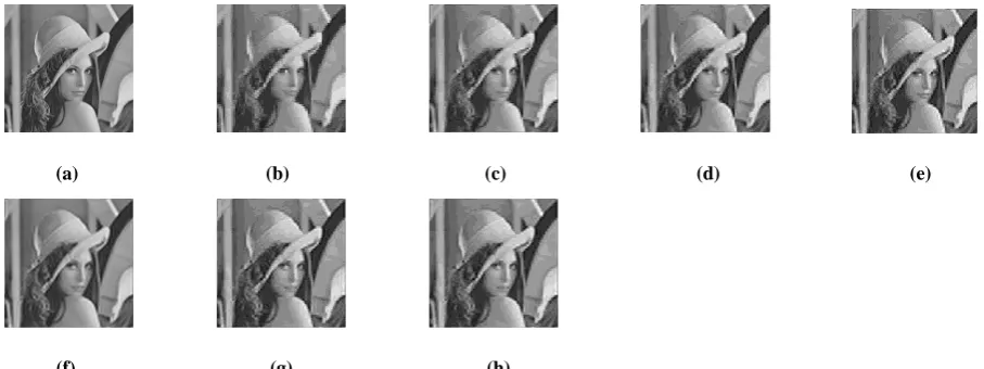
Fig 12: (a) Original ‘Lena’ image (b) Reconstructed image with db1 & BPNN (c) Reconstructed image with db2 & BPNN (d) Reconstructed image with db4 & BPNN (e) Reconstructed image with db6 & BPNN (f) Reconstructed image with db18 & BPNN (g) Reconstructed image with coiflet 5& BPNN (h) Reconstructed image with biorthogonal 6.8 & BPNN.
(a) (b) (c) (d) (e)
(f) (g) (h)
Fig 13: (a) Original ‘Lena’ image (b) Reconstructed image with db1 & RBFNN (c) Reconstructed image with db2 & RBFNN (d) Reconstructed image with db4 & RBFNN (e) Reconstructed image with db6 & RBFNN (f) Reconstructed image with db18 & RBFNN (g) Reconstructed image with coiflet 5& RBFNN (h) Reconstructed image with biorthogonal 6.8 & RBFNN.
8.
CONCLUSION
In this paper, we have proposed an image compression algorithm which integrates the features of both wavelet transform and Radial Basis Function Neural Network along with vector quantization. The images are decomposed into a set of subbands having different resolutions with respect to different frequency bands using wavelet filters. Based on their statistical properties, different coding and quantization techniques are employed. The Differential Pulse Code Modulation (DPCM) is used to compress the low frequency band coefficients and Radial Basis Function Neural Network (RBFNN) is to compress the high frequency band coefficients. The hidden layer coefficients of RBFNN subsequently are vector quantized so that without much degradation of the reconstructed image, the compression ratio can be increased.It is demonstrated from different sets of experimental results that for different wavelet filters and for a given bits per pixel (bpp), the proposed technique using Wavelet transform with RBFNN technique yields better PSNR and takes less computation time (CT) as compared to Wavelet transform with BPNN. This is because the BPNN have the limitations that it converges slowly and takes longer time to train the network. This limitation is addressed by RBFNN as it is much faster than BPNN with respect to training time, training speed and convergence. In addition, the RBFNN are less susceptible to problems with non-stationary inputs because of the behavior of the radial basis function hidden units. Furthermore, the wavelet based decomposition dramatically improves the quality of reconstructed images as compared to the neural network based technique applied on the original images. The blocking effect associated with DCT is eliminated by using wavelet decomposition. In the experiments, among the various wavelet filters tested,
Daubechies-18 resulted in slightly improved results with respect to PSNR and CT. Hence the combination of RBFNN technique and Wavelet transform along with vector quantization for hidden layer coefficients provide efficient image compression. As an extension of the proposed method, the learning vector quantization can be used instead of RBFNN.
9.
ACKNOWLEDGMENTS
The authors acknowledge the timely help and suggestion by Dr. Srinivas A, Professor and Head, Department of ECE, PESIT, Bangalore, Karnataka, India.
10.
REFERENCES
[1] P. C. Cosman, R. M. Gray, and M. Vetterli, “Vector quantization of image sub bands: A survey,” IEEE Trans. Image Processing, vol. 5, 1996, pp. 202–225.
[2] R. E. Crochiere, S. A. Webber, and J. L. Flanagan, “Digital coding of speech in subbands,” Bell Syst. Tech. J., vol. 55, pp. 1976, 1069–1085.
[3] J. W. Woods and S. D. O‟Neil, , “Sub band coding of images,” IEEE Trans. Acoust., Speech, Signal Processing, vol. 34, 1986, pp. 1278–1288.
[image:7.595.71.525.207.377.2][6] Anuj Bhardwaj and Rashid Ali, “Image Compression Using Modified Fast Haar Wavelet Transform,” World Applied Sciences Journal, vol. 7, 2009, pp. 647-653. [7] M. Mougeot, R. Azeneott, B. Angeniol, “Image
compression with back propagation: improvement of the visual restoration using different cost functions” neural networks Vol 4, No 4 1991, pp 467-476.
[8] N. Sonehara, M. Kawato, S. Miyake and K. Nakane, (1989) “Image Data Compression Using a Neural Network Model,” IJCNN con. IEEE cat. No. 89CH2765-6 Vol. 2 pp. 35-41.
[9] A. Gersho and R. M. Gray (1992), “ Vector Quantization and Signal Compression”, Boston, MA, Kluwer. [10]M. H. Hassan, H. Nait Charif and T. Yahagi, , “A
Dynamically Constructive Neural Architecture for Multistage Image Compression”, Znt. Conference on ~ Circuits, Systems and Computer, (IMACS-CS‟98). 1998 [11]Vipula Singh, Navin Rajpal and K. Srikanta Murthy,“A
Neuro-Wavelet Model Using Fuzzy Vector Quantization For Efficient Image Compression”,IJIG‟09: pp.299-320.
[12] Chi-Sing Leung, Tien-Tsin Wong, Ping-Man Lam, and Kwok-Hung Choy, “An RBF-Based Compression Method for Image-Based Relighting”, IEEE Trans. Image Processing, vol. 15, 2006, pp. 1031–1041. [13]Adnan Khashman, Kamil Dimililer, “Image
Compression using Neural Networks and Haar Wavelet” WSEAS Transactions on Signal Processing, vol. 4, may 2008, pp. 330–339.
[14]Sayood, Khalid (2000),” Introduction to Data Compression”, Second edition Morgan Kaufmann. [15]T Hong LIU , Lin-pei ZHAIV, Ying GAO , Wenming
LI', Jiu-fei ZHOU', “ Image Compression Based on Biorthogonal Wavelet Transform”, IEEE Proceedings of ISCIT 2005, pp 578-581