Design and Implementation of a Robot for Maze Solving using Flood Fill Algorithm

(1)

Design and Implementation of a Robot for Maze-Solving

using Flood-Fill Algorithm

Ibrahim Elshamarka

Department of Electrical and Electronic Engineering

Universiti Teknologi PETRONAS

31750 Seri Iskandar Malaysia

Abu Bakar Sayuti Saman

Department of Electrical and Electronic Engineering

Universiti Teknologi PETRONAS

31750 Seri Iskandar Malaysia

ABSTRACT

Autonomous navigation is an important feature that allows a

mobile robot to independently move from a point to another

without an intervention from a human operator. Autonomous

navigation within an unknown area requires the robot to

explore, localize and map its surrounding. By solving a maze,

the pertaining algorithms and behavior of the robot can be

studied and improved upon. This paper describes an

implementation of a maze-solving robot designed to solve a

maze based on the flood-fill algorithm. Detection of walls and

opening in the maze were done using ultrasonic range-finders.

Algorithm for straight-line correction was based on PI(D)

controller. The robot was able to learn the maze, find all

possible routes and solve it using the shortest one.

General Terms

Autonomous navigation, maze-solving, flood-fill algorithm,

ultrasonic sensor, PI(D) controller.

Keywords

Mobile robot, obstacle avoidance, microcontroller.

1. INTRODUCTION

In mobile robotics, autonomous navigation is an important

feature because it allows the robot to independently move

from a point to another without a tele-operator. Numerous

techniques and algorithms have been developed for this

purpose, each having their own merits and shortcomings

[1-3,8].

Maze-solving – although artificial in terms of the confine that

the robot it subjected to – is a structured technique and

controlled implementation of autonomous navigation which is

sometimes preferable in studying specific aspect of the

problem [1]. This paper discusses an implementation of a

small size mobile robot designed to solve a maze based on the

flood-fill algorithm.

The maze-solving task is similar to the ones in the

MicroMouse competition where robots compete on solving a

maze in the least time possible and using the most efficient

way. A robot must navigate from a corner of a maze to the

center as quickly as possible. It knows where the starting

location is and where the target location is, but it does not

have any information about the obstacles between the two.

The maze is normally composed of 256 square cells, where

the size each cell is about 18 cm × 18cm. The cells are

arranged to form a 16 row × 16 column maze. The starting

location of the maze is on one of the cells at its corners, and

the target location is formed by four cells at the center of the

maze. Only one cell is opened for entrance. The requirements

of maze walls and support platform are provided in the IEEE

standard [2,3].

2. RELATED WORKS

Dang and Song proposed “An Efficient Algorithm for Robot

Maze-Solving” which was based on flood-fill algorithm but

improved by reducing some steps not needed in certain cases.

As there are channels in the maze where the robot is forced to

go only straight forward, when the robot is inside these

channels, it does not need to perform all four steps of

maze-solving which is updating the wall, flooding the maze,

determining which turn to be taken and moving to the next

cell. To reduce execution time, it only flood the maze when

there is a turn [4].

“Partition-central Algorithm” is another maze-solving

algorithm where the standard 16×16 unit maze is virtually

divided into twelve partitions. The robot uses data such as its

direction and its current location to change between exploring

rules to save more time and optimize the solving process. A

simulation was developed to verify the algorithm. Test results

show that partition–central algorithm has higher average

efficiency when compared to other algorithms [5].

In another study, the discretely assigned potential levels were

discussed. Using these potential levels, the robot can

effectively make autonomous decisions to reach the goal. It

demonstrates the method of assigning and controlling these

artificial potentials to provide the most optimized path choices

while keeping the integrity of the potentials. The basic

algorithm is improved by saving information from previous

decisions that have been made [6].

3. THE MAZE AND THE ROBOT

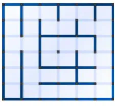
The maze designed for the robot to solve is of the size of 6×6

cells as shown in Figure 1. The actual maze constructed, as

shown in Figure 2, has a physical size of about 2.25 m

2

. The

maze was designed so that it will have two paths in order

for it to be solved. One of the paths is longer than the other.

The robot (Figure 3) must decide which one of the paths is

shorter and solve the maze through that path.

[image:1.595.372.485.605.709.2]

(2)

[image:2.595.88.248.71.367.2] [image:2.595.333.524.205.428.2]

Fig 2: The maze

Fig 3: The robot

4. ALGORITHM

Choosing an algorithm for the maze robot is critical in solving

the maze. In this exercise, flood-fill algorithm was chosen to

solve the maze due to its balance in efficiency and

complexity. There are four main steps in the algorithm:

Mapping, Flooding, Updating and Turning [2, 6-7]; which are

described in the following sub-sections.

4.1 Mapping The Maze

For the robot to be able to solve the maze, it has to know how

big the maze is and virtually divides them into certain number

of cells that can be used later in calculating the shortest path

to the destination. In this project, a maze of 6×6 cells is used.

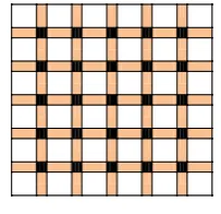
Between two cells there can be a wall. Thus, in a row of six

cells, there are five walls in between them. In total, in a row,

there are eleven units of cells or walls. This information is

stored in an 11×11 array, as shown in Figure 4. The white

units are the cells which the robot can be placed inside. The

orange units are the locations for potential walls. The black

units indicate wall intersections which are ignored by the

algorithm. The external borders of the maze are also ignored

as they are fixed boundaries of the maze. Both cells (white)

and walls (orange) are set to zero in as their initial conditions.

Fig 4: Maze-mapping Array

4.2 Updating The Wall Data

Before the robot decides where it wants to move to, it has to

check if it is surrounded by any walls in any of the three

directions: right, left and front. The robot reads the distance of

any obstacle at each direction and check if the distance in each

is more than 20 cm. The ones that exceed 20 cm are updated

as “wall” on their respective side. This is illustrated by the

flow chart in Figure 5. For the robot to update the correct wall

data, it has to know first which direction it is facing. There are

four orientations for the robot to be facing: north, south, east

or west, as shown in Figure 6. Initial orientation was set at

start and the robot keeps tracking of any changes.

Fig 5: Flowchart for updating wall location at each cell

Fig 6: Change in array locations to update the wall based

on robot orientation

4.3 Flooding The Maze

After updating the wall information for the current cell, the

robot starts to flood the matrix to find the shortest path to the

goal [6]. The flow chart in Figure 7 shows how the robot

floods the matrix and makes decision by checking one cell at

a time. It does the same for all the cells and keeps repeating

for several times until a path between the robot and the goal is

found. The algorithm assigns a value to each cell based on

how far it is from the destination cell. Based on that, the goal

cell gets a value of 1. If the robot is standing on a cell with a

value of 4, it means it will take the robot 3 steps (3 cells) to

reach the destination cell. The algorithm assumes that the

robot can’t move diagonally and it only can make 90 degree

turns.

Let Ultrasonic_Right = 0, Ultrasonic_Left = 0, Ultrasonic_Front = 0

Read Ultrasonic_Right, Ultrasonic_Left, Ultrasonic_Front

Update Wall to the Right Yes

Yes

No No

Update Wall to the Left Yes

Yes

No No Is Ultrasonic_Right less than 20 cm

Update Wall Infront Yes

Yes

No No Is Ultrasonic_Front less than 20 cm

[image:2.595.326.533.451.566.2] [image:2.595.116.218.653.751.2]

(3)

[image:3.595.59.275.71.296.2]

Fig 7: Flowchart for flooding the maze and finding the

path

4.4 Checking for Turns

[image:3.595.321.538.363.481.2]

After the robot has decided which direction it will go next, it

returns the amount of degrees it needs to turn in order to go to

the cell intended (Table 1). After turning the robot, the

algorithm updates the new orientation of the robot, i.e. facing

north, south, east or west.

Table 1. Values returned by the algorithm and its

respective turn

Degrees

Turn needed

0 No turn

90 Turn Right

180 Turn back

270 Turn left

5. HARDWARE DESIGN

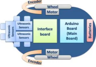
The robot has a length of 22 cm, a width of 15 cm and a

height of 15 cm. As illustrated in Fig 1, the robot is equipped

with three ultrasonic distance sensors facing front, left and

right to scan the area ahead for obstacles and specifically to

detect for walls. A wheel rotation encoder is placed near each

wheel so that the extend of how much the wheel is rotating

can be detected. With the diameter of the wheel is known, the

rotation can converted into distance traveled.

Fig 1: The robot design

5.1 Control board

Processing power is provided by an Arduino board. The

board is powered by ATmega328 which is a

microcontroller with 32 KB flash memory for storing the

code. The microcontroller can be programmed by

C-language-like “processing programming language.”

5.2 Obstacle Sensors

Three ultrasonic distance sensors were placed on the right, the

left and in front of the robot. Each ultrasonic sensor measures

the distance between the robot and any obstacle in

millimeters.

5.3 Wheel Rotation Encoder

[image:3.595.84.252.424.480.2]

Each wheel is equipped with a sensor which is basically a pair

of infra-red transmitter and receiver. By counting the

holes in the wheel and knowing the wheel diameter, the

robot can encode the distance traveled. In this case, there are

eight holes in the wheel and the wheel diameter is 7.9 cm.

That means the distanced traveled is 24.8 cm (7.9×π) when

the wheel rotates a full cycle. Figure 9 shows the counting

based on one of the wheel rotation sensors. High sensor

reading is set to one and low reading is set to zero. The frame

in black represent a detection of one cell moved, which is 16

toggles between ones and zeros.

Fig 2: Wheel Rotation Detection Curve

5.4 Motor Drive

The two wheels are driven by a pair of servo motors which are

interfaced to the Arduino board through an L293D dual

H-bridge. An L293D can drive two servo motors or two DC

motors -- which can be controlled in both clockwise and

counter clockwise direction. It has output current of 600 mA

and peak output current of 1.2A per channel. The in-built

diodes protect the circuit from back EMF (Electro Magnetic

Force) at the

outputs. Supply voltage range vary from 4.5 V to

36 V, making L293D a flexible choice for a motor driver.

6. ERROR DETECTION AND

CORRECTION

6.1 Moving in a Straight Line with a PI(D)

Controller

Due to the fact that the motors spin at slightly different speed

even when they have been calibrated, the robot tends to drift

to one side when it moves. For the robot to stay in the middle

of the corridor inside the maze, a PI controller was used to fix

the errors based on the inputs from the ultrasonic sensors. By

applying Ziegler-Nichols tuning method on the difference

between the distance detected by the left and right sensors [8].

With P-control, the ultimate gain, K

u

= 4 and the ultimate

If Cell (x,y) is not a Wall AND not a Goal

Check cells at north, south, east, and west of cell (x,y)

If boundary node has a number in it and cell (x,y) is robot location

path found! find the boundary node with the

smallest number return that direction to robot

controller If boundry node

has a number in it

Cell (x,y) = number inside boundary node + 1

END Yes Yes

Yes Yes Yes

Yes

No

Define location of Goal cell and set it to = 1 x and y start from 0 to 10 with increment of 2

x is row number and y is column number

No No

-0.2 0 0.2 0.4 0.6 0.8 1 1.2

-100 0 100 200 300 400 500 600 700

0 50 100 150 200 250 300 350

Enc

oder

Mapping

1 or

0 Amoun

t of

IR

de

tect

ed

Time

Encoder Input and Mapping

[image:3.595.63.222.600.711.2]

(4)

period, P

u

= 0.893. Table 1 shows the pertinent values derived

[image:4.595.318.533.76.205.2]

for P, PI and PID controls.

Table 1. Closed-Loop Calculations of Kp, Ti, Td

Kp

Ti

Td

P control

2 -

-

PI control

1.818 0.7445

-

PID control

2.353 0.4467

0.11167

After testing each controller and manually tuning the gain

parameters, PI controller was chosen for its smooth and

[image:4.595.56.278.230.363.2]

fast response with K

p

= 1.818 and T

i

= 0.4.

Fig 3: PI controller response

6.1.1 Choosing input for the PI(D) controller

At any one cell, relative to the walls surrounding the robot,

there are four cases. The robot can be either between two

walls, one wall on the right side, one wall on the left side or

no wall on both sides This is illustrated in Fig 4. For all cases,

the PI controller tries to keep the robot in the middle.

When the robot is in the middle, it is approximately 8 cm

away from each wall. In case the robot does not detect a wall

on its right or left side, the robot uses the wheel rotation

encoder reading to move in straight line. It counts the number

of toggles in both right and left encoder and compares them

with each other.

Fig 4: Controller input in the three cases

6.2 Turning Left or Right Using Wheel

Rotation Encoders

There are three types of turning that the robot can make. It can

either turn 90 degrees to the right, 90 degrees to the left or 180

degrees to the rear. A few tests were conducted to measure

how many toggles the encoder will count before the robot

turns 360 degrees with both wheels having the same speed

and opposite direction of rotation. Based on the results it

was determined that a 90 degrees turn would equal to 5 or 6

toggles counted and a 180 degree turn would be equal to 11

toggles.

Fig 5: Wheel rotation encoder readings for 360º

6.3 Ultrasonic Sensor Readings

As the ultrasonic sensors were exhibiting some irregular

behavior when the distance detected is below 2 cm, extra tests

were done to find the range of the correct readings. The robot

was set to move straight with the PI controller and the

readings of both left and right sensors were recorded.

As shown in Fig 6, 1680 readings were recorded with

neglecting the readings that occurred less than 30 times.

The highest occurrence was the value of 161 millimeters

which occurred 1344 times. Based on that, the value of each

sensor was chosen to be 80 mm for the robot to be in the

middle between the two walls.

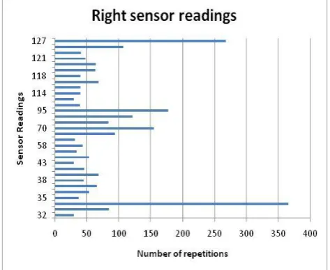
Another set of tests were done to find the accurate range for

each sensor alone. The robot was randomly moved away from

and close to a wall. 3680 readings were recorded with

neglecting the readings that occurred less than 30 times. Fig 7

shows that most of the occurrences happened at the values of

34 and 127. Based on that, the accepted range of readings

is set between 34 and 127. Any value outside this range is

neglected.

Fig 6: Sensor readings for the summation of right and left

sensors

-140 -120 -100 -80 -60 -40 -20 0 20 40

-20 -10 0 10 20 30 40 50

0 20 40 60 80 100 120 140 160 180 200

PWM PI Output

Input

-Diff

er

ence

be

tw

ee

n

righ

t a

nd

le

ft

sensor

in mm

PI controller with P=

1.818 I = 4

Input

Output

0 100 200 300 400 500 600 700

1 501 1001 1501 2001 2501 3001

Enc

oder

analogue

reading

Time

[image:4.595.316.553.454.648.2]

(5)

[image:5.595.54.290.68.260.2]

Fig 7: Sensor readings of the right sensor

7. RESULTS AND DISCUSSION

7.1 First Run

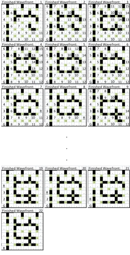
In its first run, the robot discovers the maze, map the walls

and find the target location. Each time it moves to a new cell,

its mapping matrix is updated with new information about the

existence of walls and the distance the cell is located from the

target. The distance is indicated by the number of steps

needed to move from a particular cells to the target. The first

6 steps and steps 19 & 20 are illustrated in Fig 8. Twenty

steps are required to reach the target cell. All cell and wall

data along the way are updated.

.

Fig 8: Mapping in first run requires 20 steps

7.2 Second Run

After reaching the target cell in its first run, the robot starts

heading back to its original starting point. It explores the

whole maze while continue mapping it by updating the wall

data and the distance each cell is from the target. Steps 1 to 9

and 19 to 22 are illustrated in Fig 9. It takes the robot 22 steps

to reach the starting point while seeking for an alternative

route so that the whole mapping matrix can be updated.

.

[image:5.595.315.536.176.609.2]

.

Fig 9: Return to start in second run requires 22 steps

7.3 Third run

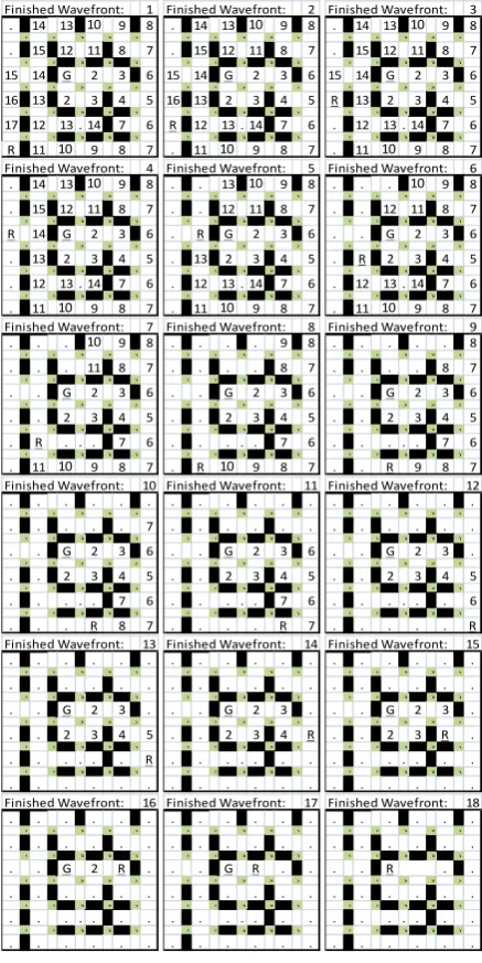
When the maze is fully mapped, the robot navigates the maze

to reach the goal through the shortest route using this data.

When deciding to move the next cell, it chooses the cell that

hold the smallest value. This is repeated until the target is

reached. This is illustrated in Fig 10.

Finished Wavefront: 1 . . . . 3 . 4 . 5 . 6 . x . x . x . x . x . . . 3 . 2 . 3 . 4 . 5 . x . x . x . x . x . 3 . 2 . G . 2 . 3 . 4 . x . x . x . x . x . 4 . 3 . 2 . 3 . 4 . 5 . x . x . x . x . x . 5 . 4 . 3 . 4 . 5 . 6 x . x . x . x . x . R W5 . 4 . 5 . 6 . 7

Finished Wavefront: 2 . . . . 3 . 4 . 5 . 6 . x _. x _. x_. x _. x _. . . 3 . 2 . 3 . 4 . 5 . x _. x _. x_. x _. x _. 3 . 2 . G . 2 . 3 . 4 . x . x . x. x . x . 4 . 3 . 2 . 3 . 4 . 5 x . x . x. x . x . R W4 . 3 . 4 . 5 . 6 x . x . x. x . x .

. W5 . 4 . 5 . 6 . 7

Finished Wavefront: 3 . . . . 3 . 4 . 5 . 6 . x _. x _. x _. x_. x_. . . 3 . 2 . 3 . 4 . 5 . x _. x _. x _. x_. x_. 3 . 2 . G . 2 . 3 . 4 x . x . x . x. x. R W3 . 2 . 3 . 4 . 5 x . x . x . x. x.

. W4 . 3 . 4 . 5 . 6 x . x . x . x. x. . W5 . 4 . 5 . 6 . 7 Finished Wavefront: 4

. . . . 3 . 4 . 5 . 6 . x _. x _. x _. x _. x _. . . 3 . 2 . 3 . 4 . 5 x _. x _. x _. x _. x _. R 2 . G . 2 . 3 . 4 x . x . x . x . x . . W3 . 2 . 3 . 4 . 5 x . x . x . x . x . . W4 . 3 . 4 . 5 . 6 x . x . x . x . x . . W5 . 4 . 5 . 6 . 7

Finished Wavefront: 5 . . . . 3 . 4 . 5 . 6 . x _. x _. x_. x _. x _. . . 3 . 2 . 3 . 4 . 5 x x _. x_. x _. x _. . R WG . 2 . 3 . 4 x x . x. x . x . . W. . 2 . 3 . 4 . 5 x . x . x. x . x . . W. . 3 . 4 . 5 . 6 x . x . x. x . x . . W. . 4 . 5 . 6 . 7

Finished Wavefront: 6 . . 4 . 3 . 4 . 5 . 6 . x x _. x _. x_. x _. . WR W2 . 3 . 4 . 5 x x _. x _. x_. x _. . . WG . 2 . 3 . 4 x x . x . x. x . . W3 . 2 . 3 . 4 . 5 x . x . x . x. x . . W4 . 3 . 4 . 5 . 6 x . x . x . x. x . . W5 . 4 . 5 . 6 . 7

Finished Wavefront: 19 . W. . W. . W. . x x x x x . W. W. . W. . x x_M xM xM x . . WG R . W. x x _. x x x . W. . . W. . x _. x _. x _. x_M x . W. . . . x _. x _. x _. x _. x _. . W. . . .

Finished Wavefront: 20 . W. . W. . W. . x x x x x . W. W. . W. . x x_M xM xM x . . WR . . W. x x _. x x x . W. . . W. . x _. x _. x _. x_M x . W. . . . x _. x _. x _. x _. x _. . W. . . .

Finished Wavefront: 1 . W. . W. . W. . x x x x x 5 W6 W. . W. . x xM xM xM x

4 5 WR . . W. x x x x x

3 W6 . 7 . 8 W. . x _. x _. x _. x_M x

2 W7 . 8 . 9 . 1 . 11 x _. x _. x _. x _. x _. G W8 . 9 . 1 . 11 . 12 Finished Wavefront: 10

. W. . W6 . 5 . 6 . x x x x _. x _. . W5 W. R W4 . 5 x x_M x

M x . x _. . 4 WG . 2 . 3 . 4 x x _. x _. x _. x _. . W3 . 2 . 3 . 4 . 5 x . x . x . x . x . . W4 . 3 . 4 . 5 . 6 x _. x _. x _. x _. x _. . W5 . 4 . 5 . 6 . 7

Finished Wavefront: 10 . W. . W6 . 5 . 6 . x x x x . x . . W5 W. R W4 . 5 x xM xM x . x . . 4 WG . 2 . 3 . 4 x x _. x _. x _. x _. . W3 . 2 . 3 . 4 . 5 x _. x _. x _. x _. x _. . W4 . 3 . 4 . 5 . 6 x . x . x . x . x . . W5 . 4 . 5 . 6 . 7

Finished Wavefront: 2 6 W7 8 W. . W. . x x x x x 5 W6 W9 1 W. . x xM xM xM x

4 5 W. 11 12 W13 x x x x x 3 W6 WR 1 W. 12 x _. x_M x . x_M x 2 W7 . 8 . 9 . 1 . 11 x _. x _. x _. x _. x _. G W8 . 9 . 1 . 11 . 12 Finished Wavefront: 10

M x . x _. . 4 WG . 2 . 3 . 4 x x _. x _. x _. x _. . W3 . 2 . 3 . 4 . 5 x . x . x . x . x . . W4 . 3 . 4 . 5 . 6 x _. x _. x _. x _. x _. . W5 . 4 . 5 . 6 . 7 Finished Wavefront: 10 . W. . W6 . 5 . 6 . x x x x . x . . W5 W. R W4 . 5 x xM xM x . x . . 4 WG . 2 . 3 . 4 x x _. x _. x _. x _. . W3 . 2 . 3 . 4 . 5 x _. x _. x _. x _. x _. . W4 . 3 . 4 . 5 . 6 x . x . x . x . x . . W5 . 4 . 5 . 6 . 7

Finished Wavefront: 10 . W. . W6 . 5 . 6 . x x x x . x . . W5 W. R W4 . 5 x xM xM x . x . . 4 WG . 2 . 3 . 4 x x _. x _. x _. x _. . W3 . 2 . 3 . 4 . 5 x _. x _. x _. x _. x _. . W4 . 3 . 4 . 5 . 6 x . x . x . x . x . . W5 . 4 . 5 . 6 . 7 Finished Wavefront: 10

. W. . W6 . 5 . 6 . x x x x _. x _. . W5 W. R W4 . 5 x xM x

M x . x _. . 4 WG . 2 . 3 . 4 x x . x . x . x . . W3 . 2 . 3 . 4 . 5 x _. x _. x _. x _. x _. . W4 . 3 . 4 . 5 . 6 x _. x _. x _. x _. x _. . W5 . 4 . 5 . 6 . 7

Finished Wavefront: 3 6 W7 8 W11 12 W15 . x x x x x 5 W6 W9 1 W13 14 x xM xM xM x 4 5 W. 15 14 W13 x x x x x 3 W6 W. R W13 12 x _. x_M xM xM x 2 W7 . 8 . 9 . 1 . 11 x _. x _. x _. x _. x _. G W8 . 9 . 1 . 11 . 12 Finished Wavefront: 10

M x . x _. . 4 WG . 2 . 3 . 4 x x . x . x . x . . W3 . 2 . 3 . 4 . 5 x _. x _. x _. x _. x _. . W4 . 3 . 4 . 5 . 6 x _. x _. x _. x _. x _. . W5 . 4 . 5 . 6 . 7 Finished Wavefront: 4

6 W7 8 W11 12 W15 . x x x x x 5 W6 W9 1 W13 14 x xM xM xM x 4 5 W. R 14 W13 x x x x x 3 W6 W. . W13 12 x _. x_M xM xM x 2 W7 . 8 . 9 . 1 . 11 x _. x _. x _. x _. x _. G W8 . 9 . 1 . 11 . 12 Finished Wavefront: 10

Finished Wavefront: 5 6 W7 8 W11 12 W. . x x x x x 5 W6 W9 1 W13 14 x xM xM xM x 4 5 W. . R W13 x x x x x 3 W6 W. . W13 12 x _. x_M xM xM x 2 W7 . 8 . 9 . 1 . 11 x _. x _. x _. x _. x _. G W8 . 9 . 1 . 11 . 12 Finished Wavefront: 10

4 5 W. . . W13 x x x x x 3 W6 W. . WR 12 x _. x_M xM xM x 2 W7 . 8 . 9 . 1 . 11 x _. x _. x _. x _. x _. G W8 . 9 . 1 . 11 . 12 Finished Wavefront: 10

M x . x _. . 4 WG . 2 . 3 . 4 x x . x . x . x . . W3 . 2 . 3 . 4 . 5 x _. x _. x _. x _. x _. . W4 . 3 . 4 . 5 . 6 x _. x _. x _. x _. x _. . W5 . 4 . 5 . 6 . 7 Finished Wavefront: 7

. W. . W. . W. . x x x x x 5 W6 W. . W. . x xM xM xM x

4 5 W. . . W. x x x x x

3 W6 W. . W. R x _. x_M xM xM x 2 W7 . 8 . 9 . 1 . 11 x _. x _. x _. x _. x _. G W8 . 9 . 1 . 11 . 12 Finished Wavefront: 10

Finished Wavefront: 10 . W. . W6 . 5 . 6 . x x x x . x . . W5 W. R W4 . 5 x xM xM x . x . . 4 WG . 2 . 3 . 4 x x _. x _. x _. x _. . W3 . 2 . 3 . 4 . 5 x _. x _. x _. x _. x _. . W4 . 3 . 4 . 5 . 6 x . x . x . x . x . . W5 . 4 . 5 . 6 . 7

Finished Wavefront: 8 . W. . W. . W. . x x x x x . W. W. . W. . x xM xM xM x

4 5 W. . . W. x x x x x

3 W6 W. . W. . x _. x_M xM xM x

2 W7 . 8 . 9 . 1 R x _. x _. x _. x _. x G W. . . . Finished Wavefront: 10

. W. . W6 . 5 . 6 . x x x x . x . . W5 W. R W4 . 5 x xM xM x . x . . 4 WG . 2 . 3 . 4 x x _. x _. x _. x _. . W3 . 2 . 3 . 4 . 5 x _. x _. x _. x _. x _. . W4 . 3 . 4 . 5 . 6 x . x . x . x . x . . W5 . 4 . 5 . 6 . 7

4 5 W. . . W. x x x x x

3 W6 W. . W. 14 x _. x_M xM xM x 2 W7 . 8 . 9 WR 13 x _. x _. x _. x_M x G W8 . 9 . 1 . 11 . 12 Finished Wavefront: 10

M x . x _. . 4 WG . 2 . 3 . 4 x x _. x _. x _. x _. . W3 . 2 . 3 . 4 . 5 x . x . x . x . x . . W4 . 3 . 4 . 5 . 6 x _. x _. x _. x _. x _. . W5 . 4 . 5 . 6 . 7 Finished Wavefront: 10

Finished Wavefront: 19 . W. . W. . W. . x x x x x . W. W. . W. . x x_M xM xM x R . W. . . W. x x x x x

3 W. W. . W. . x x_M xM xM x

2 W. . . . W. . x x_M xM xM x G W. . . . .

Finished Wavefront: 20 . W. . W. . W. . x x x x x . W. W. . W. . x x_M xM xM x

. . W. . . W. x x x x x R W. W. . W. . x x_M xM xM x

2 W. . . . W. . x x_M xM xM x G W. . . . .

Finished Wavefront: 21 . W. . W. . W. . x x x x x . W. W. . W. . x x_M xM xM x . . W. . . W. x x x x x . W. W. . W. . x x_M xM xM x R W. . . . W. . x x_M xM xM x G W. . . . . Finished Wavefront: 22

. W. . W. . W. . x x x x x . W. W. . W. . x x_M xM xM x

. . W. . . W. x x x x x

. W. W. . W. . x x_M xM xM x

[image:5.595.56.275.430.684.2]

(6)

[image:6.595.55.274.72.509.2]

Fig 10: Third run requires 18 steps

Compared to the first run where the robot was still learning

the maze, in the final run, the robot takes two less steps

because it already learned about the whole maze and knows

the shortest path to the target cell.

8. CONCLUSION &

RECOMMENDATIONS

This exercise is a study about the ability to equip a small

mobile robot with the ability to learn how to navigate in

unknown environment based on its own decisions. The

flood-fill algorithm was found to be an effective tool for

maze-solving of a moderate size. For the robot to make its decisions

it relies on inputs from several sensors, namely the ultrasonic

range sensors and wheel rotation decoders. The robot is able

to correct its orientation errors arising from its physical

motion within the maze using a PI controller.

The robot has successfully able to map the maze in the first

and second runs. In its third run it reaches its target cell

through the shortest route it has mapped in the previous two

runs.

Future works may include but not limited to studying the

robot’s maze-solving capability in a bigger and more complex

maze, in particular adaptable the robot is. The maze can be

designed and built to be reconfigurable so that the robot will

be faced with different challenge each time.

In order to improve the quality in wall detection and

self-correction, a better object sensor, such as a laser range finder,

can be employed. A laser range finder is much more costly

but provides the ability to the robot to scan its surrounding at

a wide angle plane instead of limited directional object

detection provided by ultrasonic sensors.

9. REFERENCES

[1]

Verner, I.M. and D.J. Ahlgren, Robot contest as a

laboratory for experiential engineering education. J.

Educ. Resour. Comput., 2004. 4(2): p. 2.

[2]

Mishra, S. and P. Bande. Maze Solving Algorithms for

Micro Mouse. in Signal Image Technology and Internet

Based Systems, 2008. SITIS '08. IEEE International

Conference on. 2008.

[3]

Willardson, D.M., Analysis of Micromouse Maze

Solving Algorithm, in Learning from Data. 2001,

Portland State University.

[4]

Dang, H., J. Song, and Q. Guo, An Efficient Algorithm

for Robot Maze-Solving, in Proceedings of the 2010

Second International Conference on Intelligent

Human-Machine Systems and Cybernetics - Volume 02. 2010,

IEEE Computer Society. p. 79-82.

[5]

Cai, J., et al., An Algorithm of Micromouse Maze

Solving, in Proceedings of the 2010 10th IEEE

International Conference on Computer and Information

Technology. 2010, IEEE Computer Society. p.

1995-2000.

[6]

Wyard-Scott, L. and Q.H.M. Meng. A potential maze

solving algorithm for a micromouse robot. in

Communications, Computers, and Signal Processing,

1995. Proceedings., IEEE Pacific Rim Conference on.

1995.

[7]

Jianping, C., et al. A micromouse maze sovling

simulator. in Future Computer and Communication

(ICFCC), 2010 2nd International Conference on. 2010.

[8]

Kendre, S. S., P. V. Mulmule, et al. Navigation of PIC

based Mobile Robot using Path Planning Algorithm.

International Journal of Computer Applications. 2010

[9]

Choudhury, D.R., Process Control System, in Modern

Control Engineering. 2004, PHI Learning Pvt. Ltd. p.

323-351.

Finished Wavefront: 1 . W14 13 W1 9 W8 . x x x x x . W15 W12 11 W8 7 x x_M xM xM x 15 14 WG 2 3 W6 x x x x x 16 W13 W2 3 W4 5 x x_M xM xM x 17 W12 13 . 14 W7 6 x x_M x

M x M x

R W11 1 9 8 7 Finished Wavefront: 10

M x . x . . 4 WG . 2 . 3 . 4 x x _. x _. x _. x _. . W3 . 2 . 3 . 4 . 5 x _. x _. x _. x _. x _. . W4 . 3 . 4 . 5 . 6 x _. x _. x _. x _. x _. . W5 . 4 . 5 . 6 . 7

Finished Wavefront: 10 . W. . W6 . 5 . 6 . x x x x . x . . W5 W. R W4 . 5 x x_M x

M x . x _. . 4 WG . 2 . 3 . 4 x x _. x _. x _. x _. . W3 . 2 . 3 . 4 . 5 x _. x _. x _. x _. x _. . W4 . 3 . 4 . 5 . 6 x . x . x . x . x . . W5 . 4 . 5 . 6 . 7

Finished Wavefront: 2 . W14 13 W1 9 W8 . x x x x x . W15 W12 11 W8 7 x x_M xM xM x 15 14 WG 2 3 W6 x x x x x 16 W13 W2 3 W4 5 x x_M xM xM x R W12 13 . 14 W7 6 x x_M x

M x M x

. W11 1 9 8 7 Finished Wavefront: 10

Finished Wavefront: 3 . W14 13 W1 9 W8 . x x x x x . W15 W12 11 W8 7 x x_M xM xM x 15 14 WG 2 3 W6 x x x x x R W13 W2 3 W4 5 x x_M xM xM x . W12 13 . 14 W7 6 x x_M x

M x M x

M x . x _. . 4 WG . 2 . 3 . 4 x x _. x _. x _. x _. . W3 . 2 . 3 . 4 . 5 x _. x _. x _. x _. x _. . W4 . 3 . 4 . 5 . 6 x . x . x . x . x . . W5 . 4 . 5 . 6 . 7 Finished Wavefront: 4

. W14 13 W1 9 W8 . x x x x x . W15 W12 11 W8 7 x x_M xM xM x R 14 WG 2 3 W6 x x x x x . W13 W2 3 W4 5 x x_M xM xM x . W12 13 . 14 W7 6 x x_M x

M x M x

Finished Wavefront: 5 . W. 13 W1 9 W8 . x x x x x . W. W12 11 W8 7 x x_M xM xM x . R WG 2 3 W6 x x x x x . W13 W2 3 W4 5 x x_M xM xM x . W12 13 . 14 W7 6 x x_M x

M x M x

Finished Wavefront: 6 . W. . W1 9 W8 . x x x x x . W. W12 11 W8 7 x x_M xM xM x . . WG 2 3 W6 x x x x x . WR W2 3 W4 5 x x_M xM xM x . W12 13 . 14 W7 6 x x_M x

M x M x

M x . x _. . 4 WG . 2 . 3 . 4 x x _. x _. x _. x _. . W3 . 2 . 3 . 4 . 5 x _. x _. x _. x _. x _. . W4 . 3 . 4 . 5 . 6 x . x . x . x . x . . W5 . 4 . 5 . 6 . 7 Finished Wavefront: 7

. W. . W1 9 W8 . x x x x x . W. W. 11 W8 7 x x_M xM xM x . . WG 2 3 W6 x x x x x . W. W2 3 W4 5 x x_M xM xM x . WR . . . W7 6 x x_M x

M x M x

Finished Wavefront: 8 . W. . W. 9 W8 . x x x x x . W. W. . W8 7 x x_M xM xM x . . WG 2 3 W6 x x x x x . W. W2 3 W4 5 x x_M xM xM x . W. . . . W7 6 x x_M x

M x M x

. WR 1 9 8 7 Finished Wavefront: 10

Finished Wavefront: 9 . W. . W. . W8 . x x x x x . W. W. . W8 7 x x_M xM xM x . . WG 2 3 W6 x x x x x . W. W2 3 W4 5 x x_M xM xM x . W. . . . W7 6 x x_M x

M x M x

. W. R 9 8 7 Finished Wavefront: 10

. W. . W. . W. . x x x x x . W. W. . W. 7 x x_M xM xM x . . WG 2 3 W6 x x x x x . W. W2 3 W4 5 x x_M xM xM x . W. . . . W7 6 x x_M x

M x M x

. W. . R 8 7

Finished Wavefront: 11 . W. . W. . W. . x x x x x . W. W. . W. . x x_M xM xM x . . WG 2 3 W6 x x x x x . W. W2 3 W4 5 x x_M xM xM x . W. . . . W7 6 x x_M x

M x M x

. W. . . R 7

. . WG 2 3 W. x x x x x

. W. W2 3 W4 5 x x_M xM xM x . W. . . . W. 6 x x_M x

M x M x

. W. . . . R Finished Wavefront: 13

. W. . W. . W. . x x x x x . W. W. . W. . x x_M xM xM x . . WG 2 3 W. x x x x x . W. W2 3 W4 5 x x_M xM xM x . W. . . . W. R x x_M x

M x M x

. W. . . . .

Finished Wavefront: 14 . W. . W. . W. . x x x x x . W. W. . W. . x x_M xM xM x . . WG 2 3 W. x x x x x . W. W2 3 W4 R x x_M xM xM x . W. . . . W. . x x_M x

M x M x

. W. . . . .

. . WG 2 3 W. x x x x x

. W. W2 3 WR . x x_M xM xM x

. W. . . . W. . x x_M x

M x M x

. W. . . . . Finished Wavefront: 16

. W. . W. . W. . x x x x x . W. W. . W. . x x_M xM xM x . . WG 2 R W. x x x x x . W. W. . W. . x x_M xM xM x . W. . . . W. . x x_M x

M x M x

. W. . . . .

Finished Wavefront: 17 . W. . W. . W. . x x x x x . W. W. . W. . x x_M xM xM x . . WG R . W. x x x x x . W. W. . W. . x x_M xM xM x . W. . . . W. . x x_M x

M x M x

. W. . . . .

. . WR . W. x x x x x

. W. W. . W. . x x_M xM xM x

. W. . . . W. . x x_M x

M x M x