Fast Longest Common Subsequences for Bioinformatics Dynamic Programming

Fast Longest Common Subsequences for Bioinformatics

Dynamic Programming

Arabi E.keshk

Information Menofia University

Mohammed Ossman

Institute (GEBRI)

Lamiaa Fathi Hussein

Institute (GEBRI) Menofia University

ABSTRACT

Bioinformatics applications represent an increasingly important workload to improve the programs of sequence analysis. It can be used to assign function to genes and proteins by the study of the similarities between the compared sequences. This paper introduces a modified implementation of bioinformatics algorithm for sequence alignment .The implemented algorithm is called Fast Longest Common Subsequence (FLCS). It is filling the three main diagonals without filling the entire matrix by the unused data. It gets the optimal solution but the execution time is decreased and the performance is high. To illustrate the effectiveness of optimizing the performance of the proposed FLCS algorithm and demonstrate its superiority, it is compared with Needleman-Wunsch, Smith-Waterman and Longest Common Subsequence algorithms.

General Terms

Bioinformatics. Keywords

computational biology; algorithm ; Expressed Sequence Tag ; heuristic algorithms; BLAST ; FASTA; dynamic algorithms; Needleman-Wunsch; Smith-Waterman ; LCS.

1. INTRODUCTION

In bioinformatics, a sequence alignment is a way of arranging the primary sequences of Deoxyribonucleic acid (DNA) such as Expressed Sequence Tags, Ribonucleic acid (RNA), or protein to identify regions of similarity. This similarity may be a consequence of functional, structural, or evolutionary relationships between the sequences .This field includes components of mathematics, biology, chemistry, and computer science. In bioinformatics we need some program languages such as Java, C, C++, My SQL, MATLAB and Microsoft Excel[1]. The actual process and activities within bioinformatics include the development and implementation of tools that enable efficient access to manage various types of information or the development of new algorithms (Mathematical formulas) [2]. Different alignment programs use two sequences as two strings with different length and characters arrangement. The characters are (A (adenine), C (cytosine), T (thymine), and G (guanine)) nucleotides [3]. The alignment algorithms (heuristic and dynamic) use two different types of sequence alignment, Local and Global. Local alignment is a portion or subsequence matching which is followed in Smith-Waterman dynamic algorithm, BLAST and FASTA heuristic algorithms [4].

- S1 = GCCCTAGCG GCG - S2 = GCGCCAATG

Global alignment is an end to end matching of two sequences which is followed in Needleman-Wunsch [4] and longest common subsequence (LCS) algorithms.

- S1 = G C G C – A A T G | | | | | - S2 = G C C C T A G C G

These two types of alignment are used to make a comparison between genetic sequences like Expressed Sequence Tags (EST's). EST's are small pieces of DNA sequence (usually 200 to 500 nucleotides long) that are generated by sequencing either one or both ends of an expressed gene. They are short DNA molecules reverse-transcribed from a cellular mRNA population [5],[7].

The organization of the remaining content is as follows: Section II presents an overview about bioinformatics algorithms. Section III presents the proposed algorithm (FLCS). In section IV presents the experimental work. In section V, the conclusion is illustrated. Finally,the acknowledgments is illustrated.

2. RELATED WORK

There are two types of algorithms such as: (a)- the heuristic algorithms such as BLAST and FASTA which it's advantage is ignoring the unused data from computation this speed the performance, and it's disadvantage is not found the optimal solution[3][8] .

(b)- dynamic algorithms such as (Needleman-Wunsch ,Smith-Waterman and longest common subsequences ) which it's advantage is finding the optimal alignment solution between the sequences, and it's advantages is taking more time to make the alignment this decrease the performance[3],[8],[10] 2.1 Comparison between heuristic and dynamic algorithms:

We use two real sequences such as (human insulin) with different length in the comparison between BLAST and FASTA we found that [6],[9]:

From the running of FASTA program we found:

And the approximately average of identically is = (96.3 + 78.6) % / 2 = 87.45 %.

And the approximately average of Expect value is = (7.5e-48+.035)/2= (3.75e+0.0175)

From the running of BLAST program we found

Expect-value = 8e-105 Identities = 212/220 (96%).

From the results of the two heuristic programs we found:

The expectation value of BLAST less than the expectation value of FASTA and the identities of BLAST greater than the identities of BLAST SOBLAST is more sensitive than FASTA because BLAST evaluates the result statistically and BLAST is faster than FASTA because BLAST evaluates the entire dynamic programs with the same threshold based on statistics and reduces the running time.FASTA is less sensitive than dynamic programming and BLAST because FASTA uses partial information to speed up the computation and FASTA doesn't evaluate the result statistically. The running time of FASTA is faster than dynamic programming because it doesn't evaluate the result statistically and uses partial information. The second type of programming, dynamic programming is the most sensitive result because the dynamic programming uses all information of two sequences, so the running time of the dynamic programming is slow because it computes the useless area for computing the optimal alignment[2],[8].

Table 1: Comparison between heuristic and dynamic algorithms as a general:

Algorithm Sensitivity Runtime BLAST 2 1 FASTA 3 2 Dynamic

programming

1 3

Comparison between the score of alignment (performance) for three dynamic algorithms:

2.2 Needleman-Wunsch algorithm:

The Needleman-Wunsch algorithm is a dynamic programming algorithm which finds the optimal global alignment between two biological sequences. This algorithm makes the two sequences and create two dimensional array with the length of (M*N) science M is the length of the first sequence and N is the length of the second sequence [10],[11].We can evaluate each cell by the main function with the computing formula H (i, j) is: H (i, j)=MAX{

H(i-1,j-1)+ sub(S1(i),S2(j)); H (i-1,j)+del(S1(i)); H (i,j-1)+ins(S2(j))}

The alignment between two Sequences:

sequence1=“GCCCTAGCG” and sequence2

=“GCCCTAGCG” was made as in table 2: Initialization: Gap=-2,Match=+1, Mismatch= -1. Table 2: filling Needleman-Wunsch matrix and trace back pointers [4],[11]:

G C C C T A G C G

0 -2 -4 -6

-8

-10

-12

-14

-16

-18

G -2 1 -1 -3

-5

-7 -9 -11

-13

-15

C -4 -1 2 0 -2

-4 -6 -8 -10

-12

G -6 -3 0 1 -1

-3 -5 -5 -7 -9

C -8 -5 -2 1 2 0 -2 -4 -4 -6 A

-10

-7 -4 -1

0 1 1 -1 -3 -5

A -12

-9 -6 -3

-2

-1 2 0 -2 -4

T -14

-11

-8 -5

-4

-1 0 1 -1 -3

G -16

-13

-10

-7

-6

-3 -2 1 0 0

The optimal global alignment that you get from running the Needleman-wunsch code is:

- S1 = G C G C - A A T G | | | | | - S2 = G C C C T A G C G The score of Needleman-wunsch algorithm =

(match's number*match's value)+(mismatch's number*mismatch's value)+(gap's number*gap's value)+()+() (5*1) + (3*-1) + (1*-2) = 0.

2.3 Smith-waterman algorithm:

The Smith–Waterman algorithm compares segments of all possible lengths and optimizes the similarity measure. It has the desirable to find the optimal local alignment with respect to the scoring system. The main difference between Smith-Waterman and Needleman is adding the possibility of zero value to the main function of Needleman algorithm [10][12]. The formula for computing H (i, j) becomes:

H (i-1,j-1)+ sub(S1(i),S2(j)); H (i-1,j)+del(S1(i)); H (i,j-1)+ins(S2(j))} Initialization:

Gap=0, Match=+1, Mismatch=-1,

Table 3: filling Smith-Waterman matrix and trace back pointers [12].

The optimal local alignment that you get from running the smith-waterman code is:

- S1 = GCCCTAGCG GCG

- S2 = GCGCCAATG The score of smith alignment = (3*1) + (0*-1) + (0*0) =3

2.3 longest common subsequence problems:

The longest common subsequence (LCS) problem is the third application of dynamic programming and used to find the longest common subsequence to all sequences in a set of sequences [13]. When we fill in a cell, we consider: The three values below correspond, respectively, to the values returned by the three recursive sub-problems I listed

-V1 = the value in the cell to the left -V2 = the value in the cell above

- V3 = the value in the cell to the above-left The main function in the LCS strategy: Max = {V1,

V2,

V3+1} if C1equals C2, V3 if C1is not equal to C2, where C1is the character above the current cell and C2 is the character to the left of the current cell.

Termination: We also add arrows that point pack to which of those three cells .I used to get the value for the current cell. We'll use these arrows later in "tracing back".

Tracing back to find an actual LCS:

In the tracing back step we use the cell pointers that we draw. When you have a pointer to the above-left cell, and the value in the current cell is 1 more than the value of the above-left cell, this means that the characters to the left and above are equal (match) else the characters not equal (mismatch) or gaps as shown:

Figure 1: Shows the best matches in LCS matrix with trace back and matches [13].

From the trace back:

We find the score of LCS alignment = 5. Performance:

Space: O (M*N)(we need a matrix to store all the trace back pointers ).

Time: O (M*N)( we need to fill all the cells in the matrix) Time of backing trace (M+N).

3. PROPOSED ALGORITHM

3.1 FAST longest common subsequence:

We use the same two Sequences in the new algorithm

sequence1=“GCCCTAGCG” and sequence 2

=“GCCCTAGCG”. Create a matrix of size M*N (M is the length of first sequence; N is the length of second sequence). The main steps of FAST longest common subsequences algorithm is as follow:-

1. Initialization C (0, 0) =V1= 0 Match=+1 G C C C T A G C G

C (0, 1) = C(0,0)=V1 = 0 C (j, 0) = C (0,0) = V2=0 3. Main function

Calculate the values for each cell in the three main diagonals: C (1, 1) =C (0,0)+match= V1+match=0+1=1 (i =j)

diagonal C(1,2)= max(C(0,1),C(1,1),C(0,2)) +mismatch (i ≠ j) C (0, 2) not has any value so

C (1, 2) = max(C (0, 1), C (1, 1)) = max (-1, 1) =1=1

The maximum value =left.

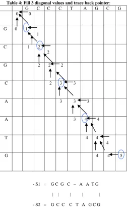
Then, follow this method to complete the three diagonal values, the matrix will be as

Table 4: Fill 3 diagonal values and trace back pointer:

G C C C T A G C G

0 0

G 0 1 1

C 1 2 2

G 2 2 2

C 2 3 3

A 3 3 3

A 3 4 4

T 4 4

4

G 4 4 5

- S1 = G C G C – A A T G | | | | | - S2 = G C C C T A G C G

From the last matrix we found that FLCS algorithm find the same optimal solution as the longest common subsequence algorithm but it ignored most unused data of the matrix so the FLCS algorithm reduce the execution time for the alignment and also increase the performance used for this alignments.

4. EXPERIMENTAL WORK:

Table 5: the table of the running time of four dynamic algorithms for the unreal sequences:

Name of algorithm s Numbers of running time

Needle man-Wunsch

Smith-Waterma n

Longest Common Subsequ ence (LCS)

FAST Longest Common Subsequ ence (FLCS)

1 828386 1188476 389326 135249 2 699740 1190778 401076

135830 3 829588 1968769 402598

138265 4 850028 1922481 404004

138401 5 672688 1207712 405876

138657 6 697936 1171042 407193

138924 7 788710 1421121 408485

139261

8 121973

6

1201100 413052 139366 9 681705 2561504 403485

139454 10 661266 1183666 425392

139544 The sum 792978

3

5368433 4060487 2605421 Average

with nanoseco nd

792978. 3

536843.3 406048.7

260542.1 Average

of millisecon d

.792978 3

.5368433 .4060487

.2605421

Smith-Waterman algorithm, and Longest Common Subsequences algorithm is = .4060487 millisecond, and finally = .2605421 millisecond by FAST Longest Common Subsequence (FLCS) algorithm.. From these values we found that our algorithms FLCS achieve the least execution time this come from ignoring the unused data of the matrix and evaluate the only three main diagonal.

Figure 2: The GUI of four dynamic algorithms and the Output alignment for the sequences S1=GCGCAATG and S2= GCCCTAGCG by using the new algorithm FLCS. The score of alignment is 5and the optimal solution is the same of LCS.

Figure 3: the diagram of the running time of four dynamic algorithms for the unreal sequences:

FLCS Case Study

:

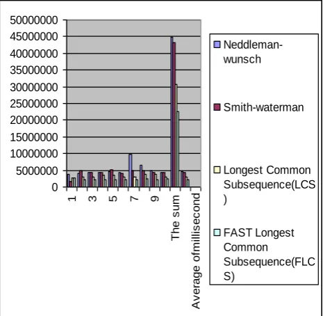
Then we apply four dynamic algorithms on the two type of human insulin such as: and EST'S sequence1 with accession number : C07137.1 and EST'S sequence2 with accession number : C07145.1 with length 231, then we found the total execution time for the alignment by using Needleman-Wunsch algorithm is 4.4839166 millisecond, and = 4.3071470 millisecond by the Smith-Waterman algorithm , and Longest Common Subsequences algorithm is = 3.0585219 millisecond, and finally = 2.2647422 millisecond by FAST Longest Common Subsequence (FLCS) algorithm.. From these values we found that our algorithms FLCS achieve the least execution time this come from ignoring the unused data of the matrix and evaluate the only three main diagonal

.

Figure 4: the diagram of the comparison between four algorithms between two sequences of human insulin (real sequences).

The running time of unreal sequences

0 1000000 2000000 3000000 4000000 5000000 6000000 7000000 8000000 9000000

1 3 5 7 9 11 13 15

The number of running time

T

h

e

v

a

lu

e

s

o

f

ru

n

n

in

g

t

im

e

Name of algorithms Numbers of running time Needleman-Wunsch

Smith-Waterman

Longest Common Subsequence (LCS)

FAST Longest Common Subsequence (FLCS)

0 5000000 10000000 15000000 20000000 25000000 30000000 35000000 40000000 45000000 50000000

1 3 5 7 9

T

h

e

s

u

m

A

v

e

ra

g

e

o

fm

il

li

s

e

c

o

n

d

Neddleman-wunsch

Smith-waterman

Longest Common Subsequence(LCS )

FAST Longest Common

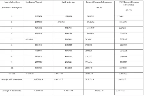
Table 6: the table of the running time fo four dynamic algorithms on the real sequences such as the EST's of human insulin:

Table 7: comparison between four dynamic algorithms.

Algorithms

Execution time of unreal sequences

Execution time of

real sequences Performance Memory locations

Big O notation

FAST Longest common subsequences

~ .2605421

millisecond

~ 2.2647422

Millisecond

High O(3M+2) as we need to fill all the matrix

O(3M+2) as we need to fill all the matrix

Longest common subsequences algorithm

~.4060487

millisecond

~ 3.0585219

Millisecond

High O(M*N)as we need to fill all the matrix

O(M+N) as

we need to fill all the matrix

Smith-Waterman

~.5368433millisecond

~ 4.3071470

millisecond Low O(M*N)as we need to fill all the matrix

O(M*N)as we need to fill all the matrix

Needleman-Wunsch algorithm

~.7929783

millisecond

~ 4.4839166

millisecond

Low O(M*N)as we need to fill all the matrix

O(M*N)as we need to fill all the matrix

Name of algorithms

Numbers of running time

Needleman-Wunsch Smith-waterman Longest Common Subsequence

(LCS)

FAST Longest Common Subsequence

(FLCS)

1 3675454 1759038 2800210 2279002

2 4055989 4782785 2948696 2214678

3 4250162 4426901 3111010 2224200

4 4355364 4449144 3660471 2265771

5 4529698 5160911 3656865 2208667

6 4468381 4031342 2908558 2223695

7 9725477 4850716 2968538 2292228

8 6405301 4901212 3787317 2316668

9 4775571 4397941 3734414 2292225

10 4357769 4311480 3009140 2330288

The sum 44839166 43071470 30585219 22647422

Average with nanosecond 4483916.6 4307147.0 3058521.9 2264742.2

5. CONCLUCION

In this paper, a modification to the implementation of Longest Common Subsequence algorithm called Fast Longest Common Subsequences (FLCS) is made. This modification depends on ignoring the unused data of the Longest Common Subsequences matrix and evaluates the only three main diagonals of the FLCS matrix. The main idea of the implementation is reducing the execution time, increasing the performance and decreasing the memory location used to make the sequence comparisons. This algorithm is based on taking the advantage of dynamic algorithms that is getting the optimal solution for the sequences alignment. It also takes the advantage of the heuristic algorithm that it is decreasing the execution time for the sequence comparison. In this implementation we use java language and the Net-beans 6.8 IDE with the JDK 1.6 to test the algorithms under the Windows Operating system with RAM 2GB.

6. ACKNOWLEDGMENTS:

First and foremost, I give my deep thanks to Allah, then I would like to thank my Husband, all my family and all Doctors who help me in this research.

7. REFERENCES

[1] Dimitris Papamichail and Georgios Papamichail2,"Improved algorithms for approximate string matching (extended abstract)"BMC Bioinformatics 2009.

[2] Wagner, R. A. and Fischer, M. J. (1974). "The string -to-string correction problem". Journal of the ACM 21 (1) , 1974: 168–173.

[3] Moulton, V., Singl, M. ALGORITHMS IN BIOINFORMATICS, 10thInternational workshop, WABI , Proceedings 2010, 20-22.

[4] Tahir Naveed, Imitaz Siddiqui, Shaftab Ahmed, “Parallel Needleman-Wunsch Algorithm for Grid”, Proceedings of the PAK-US International Symposium on High Capacity Optical Networks and Enabling Technologies. Islamabad, Pakistan, Dec 19 -21, 2005.

[5] MacIntosh, G.C., Wilkerson, C., Green, P.J. (2001). Identification and analysis of analysis of Arabidopsis expressed sequence tags characteristic of noncoding RNAs. Plant Physiol. 127(3): 765-776.

[6] Casey, R. M. (2005). "BLAST Sequences Aid in Genomics and Proteomics". Business Intelligence Network . http://www.b-eye-network.com/view/1730. [7] Lopez, C., Piegu, B., Cooke, R., Delseny, M., Tohme, J.,

Verdier, V. Using cDNA and genomic sequences as tools to develop SNP strategies in cassava (Manihot esculenta Crantz) . Theor. Appl. Genet, 2005 110: 425-431. 47.

[8] Diaz, D., Esteban, F.J., Hamandez, P. , Caballero, J.A., Dorado G. ,Galvez, S. (2011),Parallelizing and optimizing a bioinformatics pairwise sequence alignment algorithm for many-core architecture ,journal: Parallel computing-PC,VOL.37,no.4-5, pp .244-259.

[9] Source of DNA Sequences (online),National Center Biotechnology Information. Available: http://www.ncbi.nlm.nih.gov/mapview.

[10] Bin Wang, Implementation of a dynamic programming algorithm for DNA sequences alignment on the cell Matrix Architecture (online), Utah State University,

Logan, Utah. Available:

http://www.cellmatrix.com/entryway/products/pub/wang 2002.pdf

[11] Needleman, S.B. and Wunsch, C.D .(1970). "A general method applicable to the search for similarities in the amino acid sequence of two proteins". Journal of Molecular Biology.1970, 443–453.

[12] Smith, T. F. and M. S. Waterman, Identification of common molecular subsequences, Journal of Molecular Biology, 1981, 147: 195-197.

[13] Bergroth, L. , Hakonen, H. and Raita, T. "A Survey of Longest Common Subsequence Algorithms". SPIRE (IEEE Computer Society), 2000,39–48.