On testing equality of distributions of technical efficiency scores

Munich Personal RePEc Archive

On testing equality of distributions of

technical efficiency scores

Simar, Leopold and Zelenyuk, Valentin

Institut de Statistique, Université Catholique de Louvain, Belgium,

EERC, UPEG

14 December 2004

I N S T I T U T

D E

S T A T I S T I Q U E

UNIVERSIT´E CATHOLIQUE DE LOUVAIN

D I S C U S S I O N

P

A

P

E

R

0434

ON TESTING EQUALITY OF DISTRIBUTIONS

OF TECHNICAL EFFICIENCY SCORES

SIMAR, L. and V. ZELENYUK

On Testing E quality of Distributions of

Technical E fficiency Scores

Léopold Simar

*

_{and Valentin Zelenyuk}

**

Abstract

The challenge of the econometric problem in production efficiency analysis is that the very

efficiency scores to be analyzed are

unobserved

. Recently, statistical properties have been

discovered for a class of estimators popular in the literature, known as data envelopment

analysis (DE A) approach. This opens a wide range of possibilities for a well-grounded

statistical inference about the true efficiency scores from their DE A-estimates. In this

paper we investigate possibility of using existing tests for

equality of two distributions

for such a

context. Considering statistical complications pertinent to our context, we consider several

approaches to adapt the Li (1996) test to the context and explore their performance in

terms of the size and the power of the test in various Monte Carlo experiments. One of

these approaches showed good performance both in the size and in the power, thus

encouraging for its wide use in empirical studies.

Keywords: Kernel Density E stimation and Tests, Bootstrap, DE A.

Last Revision: December 14, 2004

* Institut de Statistique, Université Catholique de Louvain, Belgium.

Mailing address:

20 voie du Roman Pays, B 1348, Louvain-la-Neuve, Belgium. Tel. : + 32-10-474308, fax : + 32-10-473032.

[email protected]

.

** Institut de Statistique, Université Catholique de Louvain, Belgium and UPE G at E ROC and E ERC of “Kyiv-Mohyla Academy”, Kyiv (Kiev), Ukraine.

Mailing address:

20 voie du Roman Pays, B 1348, Louvain-la-Neuve, Belgium. Tel. : + 32-10-474311, fax : + 32-10-473032.

[email protected]

.

1. Introduction

A typical research question of many empirical studies in the area of efficiency and

productivity analysis attempts comparing differences in efficiencies among various groups

in an industry or region (e.g., private vs. public) or differences across time for the same

group(s). One way to approach this type of questions is to use non-parametric kernel

density estimator, which is becoming more and more popular in many applied areas,

including empirical economics.

Some attempts of using the kernel density estimators (KDE ) have already appeared

in efficiency analysis (see, for example, Färe and Grosskopf (1996), Simar and Wilson

(1998), Kumar and Russell (2002)). A natural way of inferring on differences in efficiency

distribution in this case would be to employ statistical tests of equality of two densities, for

example those based on the Hall (1984) central limit theorem (CLT) for degenerate

U-statistics or its extensions. These include tests proposed by Mammen (1992), Anderson et

al. (1994), Li (1996, 1999) and Fan and Ullah (1999).

The goal of this paper is to adapt one of such tests, in particular the one proposed

by Li (1996), to the context of comparing distributions of efficiency scores. The challenge

of the problem here is that the random variables (efficiency scores) whose distributions are

compared are

unobserved

. Is it reliable to use their estimates from data envelopment analysis

(DE A)—in order to test the equality of

true

distributions of

true

efficiency scores? Recent

discovery of statistical properties of this popular estimator (which before was called

deterministic) gives hopes for the positive answer, along with some warnings.

There are at least four major concerns pertinent to analysis of distributions of

DE A-estimated

efficiency scores

. One is the issue of

bounded support

of the (random) efficiency

scores distributed across population of given firms, with most of the mass often being near

the bound. The other three concerns come directly from the fact that

estimated

(rather than

the

true

) efficiencies are used. Namely, in a finite sample, the estimated efficiency scores are

biased

and

not independent

. These two problems vanish asymptotically—but with a rate of

convergence that depends on the dimension of the DE A model, which is the fourth

concern of our context. Thus, the

goal

of this paper is to address these concerns and

carefully adapt an existing test to the context of DE A-based efficiency analysis. At the end,

we suggest to researchers a reliable tool for comparing densities of true Farrell-type

2. Theoretical Model

Assume the technology of a firm

k

(

k = 1, …, n

) is characterised by the set

T

,

} :

) ,

{ (

x

y

x

can

produce

y

T

≡

, (2.1)

where N

N

x x

x =( 1,..., )'∈ℜ₊ denotes the vector of

N

inputs, while the vector of

M

outputs is denoted by y =( y₁,..., y_M)'∈ℜM₊ . E quivalently, the technology can be characterised by the

output sets

} ) , ( : { )

(

x

y

x

y

T

P

≡

∈

,

x

∈

ℜ

N₊ . (2.2)

Throughout, we assume that the technology satisfies the usual regularity axioms of

production theory, under which the Shephard (1970)

output

distance function

} { :ℜ₊N ×ℜ₊M →ℜ1₊∪ ∞ o

D , defined as

)} ( / : inf{ ) ,

(

x

y

y

P

x

D

o

≡

θ

θ

∈

(2.3)

gives a complete characterisation of the technology, in the sense that1

) ( 1

) ,

(x y y P x

Do ≤ ⇔ ∈

.

(2.4)

This function is particularly convenient as a criterion for technical efficiency of any

particular firm

k

since, roughly speaking, it gives a ‘measure’ (valued between 0 and 1) of a

distance from a point

y

k in

P

(

x

k) to the ‘upper’ boundary of

P

(

x

k), measured along the

ray from the origin. Such efficiency criterion often appears in another form, as the output

oriented

Debreu

(1951)-

Farrell

(1957) measure of

technical

efficiency

, defined for all

) ( k k

x

P

y

∈

as2

) , ( / 1 )} ( :

max{ )

,

(

x

k

y

k

y

k

P

x

k

D

_o

x

k

y

k

TE

≡

θ

θ

∈

=

. (2.5)

Formally, if we let the technological frontier be the ‘upper’ boundary of

_P

(

_x

k) _{defined as}

)} , 1 ( ),

( ),

( :

{ )

( = ∈ℜ ∈ ∉ ∀ ∈ ∞

∂ k ₊M k

λ

k

λ

x P y x

P y y

x

P (2.6)

then,

0<Do(xk, yk)<1 ⇔ yk ∈P (xk), yk ∉∂P (xk), yk ≠0, (2.7)

and thus we will call the particular observation ( k, k)

y

x

as

technically

inefficient, with

inefficiency score given by (2.5) (or its reciprocal). Alternatively, ( k, k)

y

x

is called

technically

efficient (having efficiency score equal unity) if and only if

) ( 1

) ,

( k k k k

o x y y P x

D = ⇔ ∈∂ (2.8)

Finally, D_o(xk, yk)=0, if and only if

y

k

_{= 0}

_{. Also, for further reference, we will denote}

the Farrell-type efficient ‘reference’ point for any

y

∈

P

(

x

)—the radial projection of

y

onto the technological frontier ∂P(x) with

y

∂(

x

). Formally,

) ( ) , ( / ) , ( )

(x yTE x y y D x y P x

y∂ = = _o ∈∂ (2.9)

There are also other measures of technical efficiency offered in efficiency literature.

However, the Debreu-Farrell measure seems to have been the most popular—for its

relative computational simplicity, intuitive interpretation, relationship to duality theory in

economics and, most importantly, possession of various desirable mathematical properties

(e.g., see Russell, 1990).

There are also various ways of estimating the

true

frontier of

P(x)

and the

true

efficiency score

TE

(

x,y

) for any

y

∈

P

(

x

). Apparently, one of the most popular of them is

the Data E nvelopment Analysis (DE A) estimator, which we consider in the next section.

3. The DE A estimator

In this section we focus on the class of estimators of the Farrell (1957) type (in)efficiencies

known under the general name—Data E nvelopment Analysis (DE A). There are many

variations in this class, all intending to estimate the technological

frontier

of some set-wise

characterisation of the technology and then to compute a point estimate of efficiency

scores for each observation, relative to the estimated frontier. While we will consider only

the very basic, most commonly used DE A model (that takes output orientation, assumes

variable returns to scale and free disposability of inputs and outputs), the extension to

One fundamental assumption in most DE A estimations is that all firms have

access

to the

same

technology, denoted with

T

, or its sections,P(x). This access is determined by

certain physical laws and current understanding of these laws by the humanity. This

assumption is needed to justify the estimation of

one

frontier

for all the firms in a sample,

often called the (estimated)

best practice frontier

. Although, all firms have the access to the

same technology, this does not guarantee that all firms, in a particular point in time, are

able to exploit this technology in the same way. That is, the conditions of the access to this

best-practice technology and its utilisation might be different for each firm. Namely, some

internal or external factors pertinent to each specific firm (e.g., principal-agent problems,

government interventions, particular institutions, etc) may create additional restrictions (not

always observed by researchers) on the accessibility or/and utilisation of the best practice

technology at a given moment in time. Despite optimisation behaviour, such restrictions

are likely to cause some firms or even distinct groups of them to be below the

‘best-practice’ frontier. The goal of the DE A estimator is to measure ‘how far’ each firm is from

this frontier by assigning for each firm an estimate of its (in)efficiency score, which will

represent all those restrictions on efficient use of the technology in a cumulative, residual

fashion.

A closely related fundamental assumption of the DE A estimator is that all observed

input-output combinations (

x

k

,

y

k),

k = 1, …, n

are

feasible

under

T

. In other words,

Prob

{ (

x

k,

y

k)

∈

T

} = 1,

k = 1, …, n

. This assumption implicitly allows

no

measurement

errors and

all

deviations from the frontier are assumed to be due to technical inefficiency.

However, all the data (input, output) as well as the unobserved inefficiency levels are

allowed to be random and follow some

unknown

distributions. Finally, we also assume the

true technology set,

T

, is convex.

Here, we consider the most common DE A estimator that allows for variable

returns to scale and free disposability of inputs and outputs. The

best practice frontier

under

such assumptions is estimated by an empirical analogue of (2.6) as

)} , 1 ( ),

( ˆ ),

( ˆ :

{ ) (

ˆ _{= ∈ℜ ∈ ∉ ∈ ∞}

∂P x y ₊M y P x

λ

y P x

λ

, (3.1)

where

: {

) (

ˆ M

y x

P = ∈ℜ_{+ m}

n

k

k m

k

y

y

z

≥

∑

=1

,

m = 1, ..., M,

i n

k k n

k

x

x

z

≤

∑

=1

0

≥

k

z

,

k = 1, ... , n

,

1 1

=

∑

= n k k

z

} . (3.2)

Notably, Pˆ(x) is the

smallest convex free-disposal hull

that fits the observed data and ∂Pˆ(x) is

its ‘upper’ boundary, a ‘

piece-wise linear

’ estimate of the true best-practice frontier of

P

(

x

).

The DE A estimator of individual

technical

efficiency at a fixed point (

x, y

), is

computed relative to this estimated frontier—as a solution to the following linear

programming problem (LPP)

: { max ) , ( ˆ ,..., , 1

θ

θ z zn

y x E

T = m

n

k

k m

k

y

y

z

≥

θ

∑

=1

,

m = 1, ..., M,

i n

k k n

k

x

x

z

≤

∑

=1

,

i = 1, ..., N,

0

≥

k

z

,

k = 1, ... , n,

1 1

=

∑

= n k k

z

} . (3.3)

or )} ( ˆ : { max ) , ( ˆ ,..., , 1 x P y y x E T n z z ∈

=

θ

θ

θ

The next section formally outlines the data generating process and summarises the resulting

known statistical properties of this basic version of the DE A estimator.

4. Known Statistical Results for the DE A E stimator

First, it is obvious that

Pˆ(x)⊆P(x)

, and thus

∂Pˆ(x)

is a

downward biased

estimator of

) (x P

∂

. As a result,

TEˆ(x,y)

is a downward biased estimator of

TE(x,y)

, i.e.,

) , ( ) , ( ˆ

1≤TE x y ≤TE x y , ∀ y∈Pˆ(x) (4.1)

The statistical asymptotic properties also have recently been discovered for the DE A

estimator presented above. In particular, (3.2) is consistent and is a maximum-likelihood

estimator of the frontier of

P(x)

, as shown by Korostelev et al (1995) for the univariate

(one-output or one-input) case. More recently Kneip et al. (1998) have shown consistency

and derived the rates of convergence of the DE A technical efficiency estimator (3.3) for

the multi-output-multi-input case. Gijbels et al. (1999) have discovered the limiting

distribution of DE A in the 1-input-1-output case and recently, Kneip et al. (2003) have

These statistical results require additional assumptions on the data generating

process (DGP). Let us first represent the problem by using the

polar

coordinates of

M

y

∈

ℜ

₊ defined by the modulus

ω

=

ω

(

y

)

∈

ℜ

1₊, where

ω

(

y

)

≡

y

'

y

, and the angle

1

]

2

/

,

0

[

)

(

∈

−

≡

M

y

π

η

η

, where

η

m

≡

arctan(

y

m+₁/

y

₁), if y1 >0 or

η

m

≡

π

/2, if y1 =0

for

m = 1, …, M-1

. Now, we assume:3

A1.

{ (xk, yk) : k=1,...,n} are

independent

random variables on the

convex

technology set

T

. All observations { (xk, yk) : k=1,...,n} can be partitioned into

L sub-samples

(by

some exogenous criterion) such that each sub-sample

l

(

l = 1, …, L

) represents a

distinct

sub-group l

(

l = 1, …, L

) of interest that exists in the population (e.g., public vs.

private firms in an industry).

A2.

For all

l

(

l = 1,…,L

)

,

the inputs

x

∈

ℜ

₊N has density

f

_x,l(

x

) , with compact support

N +

ℜ

⊆

ℵ

.

A3

. For all

l

(

l = 1,…,L

) and all x∈ℵ, the vector

η

≡

(

η

₁

,...,

η

M₋₁

)

has a conditional p.d.f. )

| ( ), |

(

x

f

η_{x l}

η

on

[

0

,

π

/

2

]

M−1 and the modulus

ω

has a conditional p.d.f.

) , | (

), , |

( x

fωηx l

ω

η

.

A4

. For all

l

(

l = 1,…,L

), all x∈ℵ, and all

η

∈

[

0

,

π

/

2

]

M−1

there exist constants

ε

₁

>

0

and

ε

2

>

0

such that ∀

ω

∈[

ω

( ( )),

ω

( ( ))−

ε

2]

∂ ∂

x y x

y , f(ω|η,x),l(

ω

|

η

,x)≥

ε

1,

l = 1,

…, L

, where

y

∂(

x

) was defined in (2.9).

A5

. The technical efficiency measure

TE

(

x

,

y

) is differentiable in both its vectors.

Since all the groups have access to the same technology

T

, the lower boundary of the

support )

f

_(ω|η,x),l(

ω

|

η

,

x

is the same for each group,

l = 1, …, L

. So that,

} 0 ) , | ( :

sup{ )) (

(

y

∂

x

=

ω

∈

ℜ

1₊

f

_{( |,}x_),l

ω

η

x

>

ω

ωη (4.2)

and the relation between

ω

(

y

) and the technical efficiency at (

x, y

),

TE

(

x

,

y

), is now )

( / )) ( ( ) ,

(

x

y

y

x

y

TE

=

ω

∂

ω

. (4.3)

Although the same efficiency measure (4.3) is applied for all firms in the population, the

efficiency score it yields for particular points may have different densities

f

₍ω_|η_,x_),l(

ω

|

η

,

x

)

for different sub-populations of firms

l

(

l = 1, …, L

). From now on, the superscript

l

on

the measure (4.3) will imply that this measure has been applied to a firm belonging to

group

l

(

l = 1, …, L

).

Importantly, note that A3 along with (4.3) implies the existence of a conditional (on

) ,

(

η

x

) density for

TE

l(

x

,

y

),

l = 1, …, L

(with the support [1,∞)), which we will denote

with )

f

_l(

TE

|

η

,

x

. Moreover, A4 along with (4.3), implies that

] 1 , 1 [ ,

) , |

(

TE

η

x

≥

ε

₁

∀

TE

∈

+

ε

₂

f

l ,

l = 1, …, L

. Finally, with assumptions A1-5, the

DGP, denoted with

℘

=

℘

(

P

(

x

),

g

_l(

TE

,

η

,

x

),

l

=

1,...,

L

) is completely defined through

the

joint

densities of (TE,

η

,x) ,

) ( ) | ( ) , | ( ) , ,

(

TE

x

f

TE

x

f

(| ),

x

f

;

x

g

l

η

=

l

η

ηx l

η

xl ,

l = 1, …, L

, (4.4)

each with the support Ω≡[1,∞)×[0,

π

/2]M−1×ℵ . It is this DGP that we assume has generated our sample Ξn ={ (xk, yk) : k=1,...,n} of independent observations that

are identically distributed

within

each sub-group

l

(

l = 1, …, L

) but not necessarily

across

them.

These assumptions allow us to employ the Kneip et al., (1998) theorem to claim

that the DE A estimator is consistent, and the rate of convergence is given by

) (

) , ( )

, (

ˆ

−

=

−2/(M+N+1)

p l

l

n

O

y

x

TE

y

x

E

T

. (4.5)

It is worth noting that the DGP defined above still assumes that

all

firms have

access

to the

same

technology, but the conditions of this access (“how easy it is to get to the frontier”)

are allowed to be different for different sub-groups. Such DGP can be well justified for

considering many economic phenomena. Differences in regulation regimes, ownership

structures, environments, various institutions, etc., pertinent to different groups within the

population, may have

systematic

differences in economic

incentives

or just ‘physical’

capabilities of firms in different sub-groups (sub-populations) to reach the

frontier

of the

same

technology. For example, private firms are often expected to have different incentives

for being closer to the frontier than state-owned firms. Also, firms under average-cost

under the rate-of-return regulation, or/and unregulated firms. More of philosophical

grounds for presence of inefficiency can be found in the seminal work of Liebenstein

(1966, 1992) about his concept of “X-efficiency”. The DE A thus can be viewed as an

estimator of X-efficiency, based on the Debreu-Farrell type efficiency measure. In all the

examples given above, the marginal densities that generate technical (in)efficiency (as well

as densities generating inputs and outputs) for these firms might be different across

sub-groups, while still having common best practice technology.

5. The E ssence of the Li (1996) Test for E quality of Two Densities

Although the test of Li (1996, 1999) can be used for multivariate cases, our context is

univariate and we would thus consider only the univariate version of the test in this paper.

Suppose we are interested in comparing densities of two random variables,

U

A,

U

Z

∈

ℜ

1

for which the random samples, {uA,k : k=1,...,n_A} and {uZ,k : k=1,...,n_Z}, representing the two sub-groups in a population, A and Z, respectively, are available.

Formally, letting

f

l denoting density of distribution of a random variable

U

l ₍

_{l = A, Z}

_{), our}

null and alternative hypotheses would be:

H

0: )( ) ( Z Z A

A

u

f

u

f

=

,

H

1: )( ) ( Z Z A

A

u

f

u

f

≠

, on a set of positive measure.

For testing such hypotheses, Mammen (1992), Anderson et al. (1994), Li (1996, 1999) and

Fan and Ullah (1999), have considered the integrated square difference criterion

(

f

u

f

u

)

dt

(

f

u

f

u

f

u

f

u

)

du

I

≡

∫

_A( )

−

_Z( ) 2

=

∫

_A2( )

+

_Z2( )

−

2 _A( ) _Z( )

=

∫

f

_A(

u

)

dF

_A(

u

)

+

∫

f

_Z(

u

)

dF

_Z(

u

)

−

∫

f

_A(

u

)

dF

_Z(

u

)

−

∫

f

_Z(

u

)

dF

_A(

u

) (5.1)

(which satisfies the property that I ≥0 and I =0 if and only if

H

0 is true) and suggested

slightly different empirical analogues for it as tests statistics. A particularly convenient

statistic has been proposed by Li (1996, 1999) and extended by Fan and Ullah (1999).

Using Hall (1984) CLT, Li (1996) have shown that a consistent and asymptotically normal

estimator of (5.1) is obtained by replacing the unknown distribution functions F_A(⋅) and

) (⋅

Z

(

)

∑

=

≤

≡

l l n k k l l n

l

I

u

u

n

u

F

1 , , 1 )

( ,

l = A, Z

where

I

{

X

} is the indicator function so that

I

{

X

} = 1 if statement

X

is true, and zero

otherwise, and the unknown densities in (5.1) are replaced with the non-parametric kernel

density estimators, ˆ

f

A,nA(

⋅

) and () ˆ

,nZ

⋅

Z

f

, where

∑

=

















₋

≡

l l n k l k l l l n l

h

u

u

K

h

n

u

f

1 , , 1 ) (

ˆ _,

_{l = A, Z}

_{. (5.2)}

Here, )

h

_l

=

h

(

n

_l is the smoothing parameter (bandwidth) obtained using some optimal

criterion for each sub-group

l = A, Z

,4 _while

K

is an appropriate kernel function (e.g.,

Gaussian density) and

u

is a point at which we aim to estimate the density. The latter is

often chosen to be the observed points, {uA,k : k=1,...,n_A} and {uZ,k : k=1,...,n_Z},

so that the statistic becomes

∫

∫

∫

∫

+

−

−

=

ˆ ( ) ( ) ˆ ( ) ( ) ˆ ( ) ( ) ˆ ( ) ( )

ˆ , , , , ,

,

f

u

dF

u

f

u

dF

u

f

u

dF

u

f

u

dF

u

I

_{nAnZh A AnA Z ZnZ A ZnZ Z AnA}

_















₋

Κ

+

















₋

Κ

=

∑

∑

∑

∑

= = = =

h

u

u

n

n

h

h

u

u

n

n

h

k Z j Z n k n j Z Z k A j A n k n j A A Z Z A

A , ,

1 1 , , 1 1 1 1

















₋

Κ

−

















₋

Κ

−

∑

∑

∑

∑

= = = =

h

u

u

n

n

h

h

u

u

n

n

h

k Z j A n k n j A Z k A j Z n k n j Z A Z A A

Z , ,

1 1 , , 1 1 1 1 (5.3)

Further, Li (1996) notes that the statistic based on (5.3) with the ‘diagonal’ terms removed,

i.e.,

























₋

Κ

−

+

















₋

Κ

−

=

∑

∑

∑

∑

= ≠ = = ≠ =

h

u

u

n

n

h

h

u

u

n

n

h

I

k Z j Z n k j k n j Z Z k A j A n k j k n j A A nd h n n Z Z A A Z A , , 1 , 1 , , 1 , 1 , , ) 1 ( 1 ) 1 ( 1 ˆ

























₋

Κ

−

−

















₋

Κ

−

−

∑

∑

∑

∑

= ≠ = = ≠ =

h

u

u

n

n

h

h

u

u

n

n

h

k Z j A n k j k n j A Z k A j Z n k j k n j Z A Z A A

Z , ,

1 , 1 , , 1 ,

1 ( 1)

1 ) 1 ( 1 . (5.4)

has performed better (in most Monte Carlo experiments) than the one based on the

centred version of (5.3), which may cause size distortions for finite samples. Letting

Z A n =n /n

λ

, and assuming

λ

_n →

λ

,asn_A →∞, where

λ

∈(0,∞) is a constant, Li (1996)

shows that after appropriate ‘standardisation’, the limiting distribution of (5.4) is standard

normal, ) 1 , 0 ( ˆ ˆ ˆ , , , 2 / 1 , , N I h n J d h nd h n n A nd h n n Z A Z

A ≡ →

λ

σ

(5.5)

where

σ

ˆ_λ,h is a consistent estimator of

=

2

(

∫

(

f

A(

u

)

−

f

Z(

u

)

)

du

)(

∫

Κ

(

u

)

du

)

2 2

2

λ

σ

λ ,

obtained as

























₋

Κ

+

















₋

Κ

=

∑

∑

∑

∑

= = = =

h

u

u

n

h

h

u

u

n

h

k Z j Z n k n j Z n k A j A n k n j A h Z Z A

A , ,

1 1 2 2 , , 1 1 2 2 , 1 2 ˆ

λ

σ

λ

[

∫

]

∑

∑

∑

∑

Κ

























₋

Κ

−

















₋

Κ

−

= = = =

du

u

h

u

u

n

n

h

h

u

u

n

n

h

k Z j A n k n j Z A n k A j Z n k n j Z A n Z A A Z ) ( 2 , , 1 1 , , 1 1

λ

λ

. (5.6)

6. Adapting the Li Test to the DE A Context

In this section we will be interested in comparing distributions of

efficiency

scores

for two

sub-groups, A and Z, in an economic system (industry, country, etc). Let us first check the

satisfaction of regularity conditions used in Li (1996). According to A1-A5, the

true

technical efficiency scores in each sub-group, {TEA,k : k=1,...,n_A} and

} ..., , 1 :

{ Z,k _Z

n k

TE = , are distributed

independently

(and identically within each sub-group)

with densities f_A(⋅) and f_Z(⋅), respectively. (Contemporaneous correlation is allowed between the two samples.) In real world, however, the true independent efficiency scores

are unobserved but estimated with DE A, which are independent only asymptotically, while

in finite samples they are dependent (by construction) with unknown structure of

dependency. It is thus not clear whether the original Li-test would perform well in this

context. The assumption A1-A5 also ensure that

f

A

(

⋅

)

and fZ(⋅) are continuous and

bounded in ℜ1 and have some distribution functions

F

A

(

⋅

)

and FZ(⋅), respectively. For

simplicity, we will also use the Gaussian kernel to estimate these densities, which is a

Since construction of the test statistic essentially involves formulas for kernel

density estimator, the special issues pertinent to the kernel density estimation in DE A

context, might be important in the Li-test context as well. The first is the issue of

bounded

support

in density estimation, since it is known that the standard kernel density estimator is

inconsistent at the boundary. This can easily be circumvented by using the Schuster

(1985)-Silverman (1986) reflection method, which provides the consistent estimator 5











≥

























₋

₋

+













₋

≡

∑

₌ . , 0 , ) 2 ( 1 ) ( ˆ 1

otherwise

b

u

h

u

u

b

K

h

u

u

K

nh

u

f

n k R i R i R R (6.1)

A natural question is whether one also needs to use this (or other) method for adapting the

Li-test to the DE A context. In his Monte Carlo experiments, Li (1996) have considered

application of his test to the case of Uniform density and obtained good performance. Our

case is somewhat more severe than the uniform: most of the mass might be very close to

the bound and we know that the estimator for such case can give very poor fit. However,

note that for symmetric kernels, the estimation procedure (6.1) is equivalent to estimating

) ( ˆ

2f u using (5.2) from the original data {

u

₁,...,

u

_n}, on the bounded support, but with a

bandwidth selected from the

reflected

data {

u

1,...,

u

n,2

b

−

u

1,...,2

b

−

u

n} , which we denote

as h_R. Hence, the reflected analogue of (5.3), will be twice as much as (5.3), given h_R, i.e.,

d h n n nd h n n R d h n n R nd h n n R h n

nA Z R

I

A Z R

I

A Z R

I

A Z R

I

A Z R

I

, , , ,

, , , , , , ,

, ˆ ˆ 2ˆ 2ˆ

ˆ

_≡

₊

₌

₊

_{, (6.2),}

where _ndR_{n h}

R Z A

I

ˆ ,, , is part of

R h n nA Z R

I

ˆ , , , involving only diagonal terms of it. Using the Hall

(1984) theorem, similarly as Li (1996), we get that (for a univariate case)

) 1 , 0 ( ˆ ˆ 2 ˆ ˆ ˆ , , , 2 / 1 , , , , 2 / 1 , ,

N

I

h

n

I

h

n

J

d h nd h n n R A h R R nd n n R A nd R n n R R Z A R Z A Z

A

≡

=



→

λ

λ

σ

σ

(6.3)

where we have also used the fact that ˆ2_{, ,} 2ˆ2

R R λ,h

h

R

σ

σ

λ

=

. Thus, the statistic based on

reflection method is essentially the same as the original Li (1996) test, with the difference

being a factor of 2 and the fact that the bandwidth used in estimation of statistic is

obtained from the data with reflection rather than the original data. As we will see in

Monte Carlo experiments, (6.3) does not improve upon the original Li (1996) statistic in the

sense that both of them have similar performance (e.g., bootstrap estimated sizes of the

test are not significantly different from each other and from the true sizes.) This suggests

that despite the fact that reflection method is useful in density estimation

per se

, it is

essentially not needed for adapting the original Li-test to the case of comparing the

densities with bounded support (with a lot of mass near the bound).

The second is the issue of using not the true random variables whose densities we

want to compare, but their estimates which, in finite samples, are downward-biased and

dependent.6 The Li (1996) test is

asymptotic

in nature, so the problem of the finite-sample

bias and dependency of DE A-estimated efficiency scores is mainly an empirical problem.

For example, it might be that due to high sampling variation or noise from the DE A

estimation, researchers may run into the

type-I

(incorrectly reject the true Ho) and

type-II

(failing to reject the incorrect Ho) errors more often than they would under the (unrealistic)

situation when the true efficiency scores are known. If so, such inference may bring

researchers to misleading conclusions and incorrect policy recommendations. It also might

be that since the bias problem influences, in the same fashion, the estimation of

both

densities under comparison, then the overall ‘damage’ might happen to be not so

significant for the test itself, especially under the null. Experimental evidence through

Monte Carlo experiments is clearly needed here.

Overall, even in large samples, and especially in finite samples, the performance of

the original Li-test adapted to the DE A context using the (first order) Normal

approximation might be far from desirable. As a result, carefully designed bootstrap may

be needed to improve its performance. In fact, Li (1999), using the true random variable,

give some Monte Carlo evidence that the bootstrap provides better inference than the use

of normal tables. This shall not be surprising, given the asymptotically pivotal nature of the

statistic. In the next section, we will consider several bootstrap algorithms in the aim of

suggesting the most reliable one for empirical research.

7. Bootstrapping the ‘adapted to DE A context Li-test’

It is now known that the naïve bootstrap is inconsistent for the individual DE A-estimates

(e.g., see Simar and Wilson, 2000 for details). On the other hand, Kneip et al. (2003) had

proven consistency property of the

sub-sampling

bootstrap—when the sub-sample size is

smaller than the original sample size. They also provide Monte Carlo evidence that earlier

suggested

smooth

bootstrap is an approximation of the consistent sub-sampling bootstrap.

In principle, we could use the two-stage approach: first correct for the bias in the DE A

efficiency estimates using one of the consistent versions of bootstrap for DE A and then, at

the second stage, use these bias-corrected estimates in the Li-test for comparing the true

densities of the true efficiency scores. Analysing such approach under various

Monte-Carlo scenarios is very computer-time-consuming, even with modern computers (just one

bootstrap bias-correction procedure may take several hours, since it requires LP

optimisation for each efficiency score). Instead, we will use (slightly modified) sample of

original DE A estimates for using in the Li-statistic, which in turn we bootstrap to obtain

p-values. Results from various Monte Carlo scenarios yield evidence of good performance of

such algorithms under moderate dimensions of DE A model, requiring much less computer

time than the tests that would involve bias correction.

Specifically, we will analyse two bootstrap alternatives. The first one, call it

Algorithm I

, is based on computation and bootstrapping the Li-statistic using the sample of

DE A-estimates

trimmed

from those that are equal to unity, i.e., just ignore the ‘spurious

ones’ for the sake of the test. The second one, call it

Algorithm II

, is based on computation

and bootstrapping the Li-statistic using the sample of DE A-estimates where those equal to

unity are ‘

smoothed

’ away from the bound by adding a small noise, say within 5%-quantile of

the empirical distribution of ˆ( k, k)

y x E

T ignoring those equal unity, but of order smaller than the noise of estimation (suggested by the rate of convergence). Formally, the

smoothing is made by

 

 _{+ =}

=

otherwise y

x E T

y x E T y

x E T y

x E

T _{k k}

k k k

k k k

k

), , ( ˆ

1 ) , ( ˆ , ) , ( ˆ ) , (

ˆ*

ε

(7.1)

where

ε

k =Uniform(0, min{n−2/(M+N+1),a} ),

a

is the

α

-quantile of the empirical

distribution of _TEˆ(_xk, _yk) _{ignoring those equal unity. For the sake of reader’s} convenience, the complete description of both bootstrap algorithms for Li-statistic in DE A

context is given in the next table.

< Insert Table 1 here >

The obtained

bootstrap

estimates of DE A-adapted Li-statistic can then be used to

estimate the

p-value

of the test, by using

{

}

∑

=

>

=

−

B

b

nc n n b nc

n

nA Z

J

A Z

J

I

B

value

p

1

, ,

*

, ˆ ˆ

1

ˆ , (7.2)

8. Monte-Carlo Investigation of the Size of the Test

The goal of this section is to illustrate the methods described above on some examples

where we know the ‘truth’ and thus can get a feeling of the performance of the proposed

techniques.

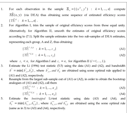
8.1. Simulated E xample 1: Does Reflection Improve the Size of the Test?

In efficiency analysis, researchers often expect (or assume) efficiency distributions are

skewed so that most of the mass is close to efficient bound (unity in our case) with a

diminishing tail towards higher inefficiency—manifesting economic agent’s tendency to

strive for full efficiency or a level near it. A typical example for such a distribution can be

constructed from normally distributed variable, truncated at unity. Here, we assume that

the

true

technical efficiency is

TE

l,k

=

1

+

u

l,k, where , ~ ( l, l2)

k l

N

u

+

µ

σ

,

l = A, Z

, where 0

= = Z

A

µ

µ

and

σ

A

=

σ

Z

=

1. For this example, assume that the true (realisations) of

efficiency scores are known and our goal is to see if, in such ideal conditions, the

application of the reflection principle to the original Li-test would bring any improvement

100, 200} with MC = 1000 and B = 400 (which would allow also comparing our results to

those of Li, 1999; For real data, we would recommend

B

largerthan 1000). We estimate

four values of the true (nominal) sizes: { 0.01, 0.05, 0.10, 050} .7

From Table 2, one can see that the bootstrap estimated sizes of the

original

Li-test

applied to ‘observed’ (in simulation) true efficiency scores are already very close to the true

sizes, statistically insignificantly different from them, and so is the test that accounts for

boundary issue via the reflection principle. As a result, in our future investigations we will

not worry about the reflection issue.8

< Insert Table 2 here >

8.2. E xample 2: Algorithm I vs. Algorithm II in Different Dimensions

Now we consider the main problem of the paper: the case when the true efficiency scores

are

not

observed but estimated via DE A. And, the goal of the experiment is to see what

approach performs better: (i) trimming the estimates that equal to unity, (Algorithm I), or

(ii) smoothing them according to (7.1), with

α

= 5% (Algorithm II). DE A is a

non-parametric estimator and the shape of technology does not matter much for it, as long as it

satisfy the regularity assumptions on DE A (especially convexity). What matters the most,

however, is the dimension of the DE A problem (number of inputs and outputs in DE A

specification), as suggested by the rate of convergence (4.5). So we will consider only one

technology type, Cobb-Douglass, but in different dimensions—to investigate an impact of

curse of dimensionality. Specifically, assume that the true technology frontiers are

characterised by the Shephard’s output distance function of the following forms,

) /(

) ,

( 02.5

3 . 0 1 * *

x x y y x

Do = (8.1)

) /(

) ,

(x y* y* x₁0.1x₂0.15x₃0.2x0₄.05

Do = (8.2)

) /(

) ,

(x y* y* x₁0.1x₂0.15x0₃.2x₄0.05x₅0.25x₆0.07x₇0.08

D_o = (8.3)

7 _{The 95% Monte-Carlo confidence intervals (with 1000 replications) for these values would be} approximately { (0.0037, 0.0163), (0.0362, 0.0638), (0.081, 0.119), (0.4684, 0.0316)} , respectively.

where

y

* is the technically efficient output level, given input levels (

x

1,

x

2)', which we

assume are both coming from

Uniform

(

0,1

) distribution for each sub-group

.

The ‘observed’

output

y

(for each group) is obtained as lk lk

TE

y

y

,

=

*/ , . Here, we assume that the null is

true, in particular,

µ

_A =

µ

_Z =0 and

σ

_A

=

σ

_Z

=

0.3, thus ( l,k)

≈

1.24

TE

E

, and consider

four sub-sample sizes:

n

A =

n

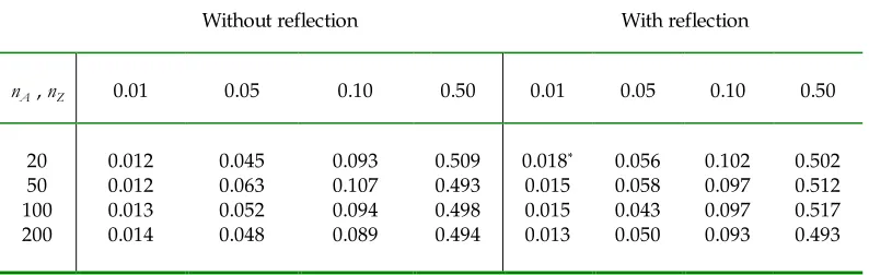
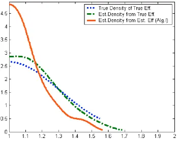
Z = { 20, 50, 100, 200} , with MC = 1000 and B = 400.

In Figure 1, we produce three curves for a typical Monte-Carlo replications for this

scenario and in Figure 2 we have

µ

=

0.3 and

σ

=0.3. For both cases we have

n

= 50 and

technology (8.1). The dotted curve is the true density of the true efficiency scores. The

dash-dotted curve is the corresponding estimated density when the true efficiency scores

are observed, but their density is estimated via (6.1). Finally, the dashed curve is estimated

density when the true efficiency scores are unobserved but their density is estimated via

(6.1) from the DE A-estimates (except those equal unity)—the situation faced in reality by

practitioners. We use Gaussian kernel and Sheather and Jones (1991) method for

estimating

h

. One can clearly see the empirical issue raised in our paper: the problem of

using the DE A-estimates in place of the true but unknown efficiency scores.

< Insert Figure 1 Here> < Insert Figure 2 Here>

The ‘double’ estimation (of efficiency and of density) produces density estimate that may

look quite differently than the true density. In particular, the downward bias of the DE

A-estimates results in ‘too much’ mass allocated near the bound. The density estimation based

on the smoothed DE A estimates via (7.1) was allocating even more mass close to the

bound (figures for which are not presented for the sake of space). This is of course only

one replication presented that seemed typical to us. In some draws the fit was better, in

others it was worse. Increase in sample size certainly tended to improve the fit, while

increase in the dimension tended to worsen it. All this naturally raises questions and

perhaps serious concerns about reliability of Li-test for the case of comparing distributions

of efficiency scores that are unobserved but estimated via DE A, which we now analyse.

The results of our size investigation, presented in Table 3, are quite interesting and

encouraging. For the case of two inputs, results presented in Table 3 suggest that (under

the null) the estimated sizes for both algorithms are in most cases insignificantly different

Algorithm I was significantly different from its nominal value of 0.01. When we increase

dimension to 4 and 7 inputs, we sometimes could not obtain the bootstrapped p-values for

Algorithm I. This is because the number of observations on the frontier (to be deleted in

Algorithm I) increases with the dimension, resulting in too few observations or even in

estimated variance being very close to zero for some bootstrap samples. The estimated

sizes for Algorithm II for these cases, however, were mostly insignificantly different from

the nominal sizes. In case when it was possible to compute the p-values for both

Algorithm I and II, their performance was very similar. On this basis, we conclude that the

two bootstrap algorithms, I and II, for the Li (1996, 1999) test adapted to the DE A context

are reliable in terms of size of the test, with Algorithm II being more robust to the curse of

dimensionality problem and, in our experiments, always had correct size at 5% and 10%

levels, which are those most commonly used in practice.

< Insert Table 3 here>

9. Monte-Carlo Investigation of the Power of the Test

The goal of this section is to investigate the power of the test (i.e., probability of correctly

rejecting the false null hypothesis) in different dimensions of DE A model. We will

compare the power of test based on Algorithm II

vs.

the power of the test based on the

true

efficiency scores, which are known in Monte-Carlo study and can be considered as a

benchmark for comparison. In particular, we investigate the power of the test in the case

of different modes/means (before truncation) of efficiency distributions. Here we take the

set-up of simulation example 1, but assume

µ

_A

=

0,

σ

_A

=

0.4, while

} 1 , 9 . 0 ,..., 9 . 0 , 1 { ,

∈

−

−

=

δ

δ

µ

Z and

σ

Z

=

0.4. So, when

δ

=

0, the null hypothesis is

true. We consider three sample sizes:

n

A =

n

Z = { 20, 50, 100} , with MC = 1000 and B =

400. For the insight onto the impact of curse of dimensionality we present results for

several technologies. In particular, for the case of 20 observations in each group we use

(8.1), (8.2) and two more technologies,

) /(

) ,

(x y* y* x₁0.1x₂0.15x0₃.2

Do = (9.1)

and

) /(

) ,

(x y* y* x₁0.1x₂0.15x₃0.2x0₄.05x₅0.25

D_o = , (9.2)

while for the case of 50 and 100 observations in each group we use technologies defined in

First of all, it must be quite intuitive that the power functions for algorithms II shall

outperform that of I, unless too much noise is added. This is because algorithm II

always

uses more observations than algorithm I (which ignores observations equal unity),

especially for large dimensions, and this was confirmed in all our simulations (not

presented). Thus, we only present the power functions for algorithm II, where DE

A-estimates are obtained under different dimensions and compare them to the case when the

true (realizations) of efficiency scores are used in the original Li (1996, 1999) test.

For convenience, we present the results by plotting the estimated power functions

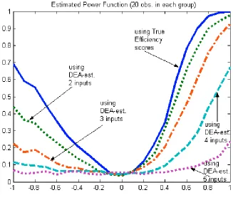
(for nominal size of 0.05) in Figures 3-5, while numerical values are reported in the table in

the appendix. Remarkably, although the size of the test was very good relative to the true

(nominal) size even for 20 observations in each sample, the estimated power functions

suggest that the power of the test for such a small sample as 20 is quite low, especially

when the dimensions of the DE A model is high. Note that the power functions for 20

observations in each group are very asymmetric with a flatter left tail—warning about

reliability of the test conclusions based on such small samples, even for the case when the

true

efficiency scores are used (in original Li test).

The power function for the algorithm II based on 2-input-1-output DE A-estimates

of efficiency mimics the asymmetric shape of that based on

true

efficiencies, getting quite

close to this ‘ideal’ when the two distributions have different modes (after truncation), but

worse for the case when the two distributions being different are having the same (unity)

mode. This pattern is repeated for higher dimensions as well, such that the higher the

dimension the worse is the power—manifesting the curse of dimensionality problem of the

DE A estimator. Again, this problem is especially clear when the two distributions have the

same mode. The case of 5-input-1-output case with 20 observations in each group yields

the power function that is virtually flat—alerting about the danger of misleading

impression about equality of distributions from such large dimension relative to such small

samples.

< Insert Figure 3 here>

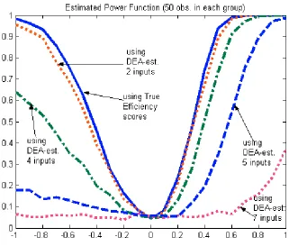
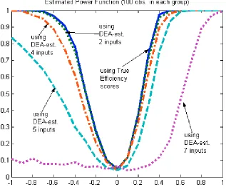
Observing and comparing Figures 4 and 5 to Figure 3 brings some optimistic

feeling. The pattern is similar, but the larger the sample size the less asymmetry and the

steeper are the power functions. The curse of dimensionality problem reduces with

increase of the sample, as it is expected to be. For example, for the case of 100

case becomes almost identical with the power function for the case when the true

efficiency scores had been used. E ven the power function from the estimates in the

4-input case also becomes much closer to that based on the true efficiency scores—when we

compare 100 observations case with 50 observations case and certainly relative to 20

observations case. For 5-input model, the performance of the test improves for 50

observations and becomes reasonably good for 100 observations case (but the left tail still

lags behind).

< Insert Figure 4 here> < Insert Figure 5 here>

Importantly, the power function from the estimates in the 7-input case is quite

unsatisfactory even for 100 observations case (very flat). The intuition for this is in the fact

that high dimension of DE A model relative to the sample size leads to many observations

being on the estimated frontier (due to being ‘unique in their own way’) in both groups and

thus smoothing such estimates according to mechanism (7.1) ‘homogenises’ a big chunk of

the two samples. So the resulting smoothed samples look much more the same than their

populations are and the test statistic thus would have less power than it should when the

true efficiency scores are (unrealistically) observed.

An issue in itself deserving special attention is the asymmetry of the power

functions, which luckily vanishes when the sample size increases. The reason for this

asymmetry is in the nature of the distributions analysed. Namely, we deal with

distributions truncated on one side, highly asymmetric and, as can be observed from the

figures, the true alternative hypothesis that presumes mode greater than unity in one

distribution vs. unity-mode for another is more empirically identifiable than when

comparison is between two asymmetric distributions with unity modes. (Additional Monte

Carlo experiments for comparison of symmetric distributions confirmed this conjecture.)

In other words, the test has greater power in distinguishing distribution with what Simar

and Zelenyuk (2003) called as tendency for ‘pathological inefficiency’ (non-unity mode) vs.

distribution where firms are having tendency to full efficiency, represented by (unique)

10. Conclusion

The goal of this paper was to provide researchers with a reliable tool for testing equality of

distributions of Farrell-type

efficiency

scores between groups of decision making units

(plants, firms, etc) within a population (industry, country, region, etc). We have considered

two major specifics pertinent to analysis of distributions of DE A-estimated efficiency

scores and investigated ways to incorporate them to testing procedure. One is the issue of

bounded support

of the distribution of efficiency scores. The other is the usage of

estimated

rather than the

true

efficiencies, which are then used to

estimate

the

true

densities of

true

efficiency scores. Such estimates are biased and not independent—problem that vanishes

asymptotically, but with a rate of convergence that depends on DE A dimension.

We incorporated this knowledge into considering various algorithms for testing

equality of densities based on Li (1996, 1999) test. We demonstrated that the reflection

method is unnecessary here. We also considered two algorithms that handle the problem

of ‘spurious mass at the bound’: Algorithm I simply ignores the boundary estimates and

Algorithm II smoothes such estimates by adding uniform noise of order smaller than the

speed of convergence of the DE A estimator. Limited Monte Carlo evidence suggests that

both algorithms have good size (insignificantly different from nominal one). However,

Algorithm II was more

robust

to the increase in dimension.

Finally, the results of investigation of the

power

of the test suggest that, for relatively

small dimensions of DE A model (e.g., 2 or 3 inputs and 1 output for 50 observations in

each group), the power is quite good—close to the ‘ideal’ case, when

true

efficiency scores

are used in testing. However, the curse of dimensionality problem (of the DE A estimator)

is indeed a problem here: When the dimension is high relative to the sample size (e.g., 5

inputs, 1 output, for 20 observations in each group) then the power of the test is quite low.

Very low power (although correct size) was also identified for 7-input-1 output case for 50

(and to some extent even for 100) observations in each group, especially when compared

distributions in both groups have unique unity mode (no pathological inefficiency).

Overall, we conclude that given no abuse with the dimension of DE A model

relative to the sample size, the Li (1996) test, adapted via our Algorithm II, is a reliable tool

for testing equality of distributions of unknown but DE A-estimated efficiency scores. For

the sake of brevity we had not presented an application here, but an interested reader is

referred to recent applications of this method to Henderson and Zelenyuk (2004) and

References

Anderson, N., Hall, P. and Titterington, D.M. (1994), “Two Sample Test statistics for Measuring Discrepancies between Two Multivariate Probability Density Functions Using Kernel-based Density E stimates,”

Journal of Multivariate Analysis

, 50, 41-54.

Debreu, G. (1951), “The coefficient of resource utilization,”

Econometrica

, 19, 273-292.

E fron, B. (1979), “Bootstrap methods: another look at the jackknife,”

Annals of Statistics

7, 1-26.

Farrell, M.J. (1957), “The Measurement of Productive E fficiency,”

Journal of Royal Statistical

Society

, Series A, General, 120, part 3, 253-281.

Fan, Y. and A. Ullah (1999) “On Goodness-of-fit Tests for Weakly Dependent Processes Using Kernel Method.”

Journal of Nonparametric Statistic

s 11(1–3), 337–60.

Gijbels, I., E . Mammen, B.U. Park and L. Simar (1999), "On E stimation of Monotone and Concave Frontier Functions",

Journal of the American Statistical Association

94, 220-228.

Hall, P. (1984), “Central Limit Theorem for Integrated Square E rror of Multivariate Nonparametric Density E stimators,”

Annals of Statistics

, 14, 1-16.

Hall, P. (1992),

The Bootstrap and Edgeworth Expansions

, Springler, New York.

Kneip, A., L. Simar and P. Wilson (2003a), “Asymptotics for DE A E stimators in Non-parametric Frontier Models”,

Discussion Paper #0317, Institut de Statistique,

Université

Catholique de Louvain

, Belgium

Kneip, A., B. Park and L. Simar (1998), “A Note on the Convergence of Nonparametric DE A E stimators for Production E fficiency Scores”,

Econometric Theory

14, 783-793.

Korostelev,A., Simar,L. and Tsybakov, A.B.(1995), “On estimation of monotone and convex boundaries,”

Publ. Statist. Univ. Paris

XXXIX 1, 3 –18.

Li, Q. (1996), “Nonparametric Testing of Closeness between Two Unknown Distribution Functions,”

Econometric Reviews

15, 261-274.

Li, Q. (1999), “Nonparametric Testing the Similarity of Two Unknown Density Functions: Local Power and Bootstrap Analysis,”

Nonparametric Statistics

11, 189-213.

Liebenstein, H. (1966). “Allocative E fficiency vs. ‘X-E fficiency’,”

American Economic Review

56, 392-415.

Leibenstein, H. and S. Maital (1992). “E mpirical E stimation and Partitioning of X-Inefficiency: A Data-E nvelopment Approach,”

American Economic Review

82, 428-433.

Mammen, E . (1992),

When Does Bootstrap Work? Asymptotic Results and Simulations

, Springler, New York.

Pagan, A. and A. Ullah (1999),

Nonparametric Econometrics

, Cambridge University Press. Park, B. Simar, L. and Ch. Weiner (2000), "The FDH E stimator for Productivity E fficiency