Currency substitution in Romania

(1)

Munich Personal RePEc Archive

Currency substitution in Romania

Lazea, Valentin and Cozmanca, Bogdan Octavian

National Bank of Romania

May 2003

Online at

https://mpra.ub.uni-muenchen.de/19813/

(2)

C

U

R

E

N

C

Y

S

U

B

S

T

I

T

U

T

I

O

N

I

IN

N

R

RO

OM

M

A

NI

N

IA

A

∗

Valentin Lazea

1

– Chief Economist, National Bank of Romania

Email:

Bogdan Octavian Cozmânc

ă

1

– economist, National Bank of Romania

Email:

May 2003

* Paper presented at a conference organised by the Bulgarian National Bank in June 2003

1

(3)

Abstract

The aim of this paper is to investigate the currency substitution phenomenon in Romania. We present the evolution of the DI (Dollarization Index) as it is defined by the IMF, the situation on the liabilities side and that of the banking sector. We assess the way in which the traditional functions of money have been affected by currency substitution. In the final part of this paper a demand for money function is estimated for Romania for a period between 1997:06—2003:03. This demand for money clearly demonstrates the existence of currency substitution between the domestic and foreign currencies. Also we test the stability of the model and conclude that despite a turbulent economic medium the demand for money function is stable.

Keywords: currency substitution, money demand, cointegration, error-correction model, Romania

(4)

I. The currency substitution phenomenon

Monetary instability during the transition process from a command economy towards a market one, the increased openness of the economy and the development of trade with the EU, induced a considerable increase in currency substitution in most of the Eastern European economies.

Currency substitution has important effects not only on monetary policy but also on fiscal policy. When currency substitution is widespread, the effective money supply is much larger than the domestic money supply and is, moreover, less easily controlled by the monetary authority because of the public’s tendency to substitute foreign for domestic currency. In such an environment for example, an inflationary fiscal policy – imposing an implicit tax on domestic monetary assets, will be ineffective, monetary policy is prone to a more volatile velocity of money, lower monetary depth is also a consequence, part of the segniorage revenues is lost, not to mention that foreign cash transactions reduce the cost of tax evasion and facilitate participation in the “underground” economy. It is clear that formulating macroeconomic policy in such circumstances is not an easy task.

A decision to adopt euro by the transition economies can be due to different advantages that can arise, such as: a greater stability of the exchange rate versus the Euro zone area (and incentives for foreign investment), the risk of speculative attacks on the domestic currency is virtually eliminated, and the need for large foreign reserves is diminished. Also a possible pro argument is that the process is in theory reversible.

(5)

A further key problem is the separation, in the research of currency substitution, of currency substitution and currency substitutability (the ability to be substituted) presented by Giovannini and Turtelboom (1992) in their paper which reviews the literature on the subject. This distinction creates two separate streams of research. The study of currency substitutability would explore its potential effect, domestically and internationally, on variables of interest to economists and policymakers. The study of substitution would explore the size and the potential causes of the (partial) replacement of one currency with another, and from them extract a better understanding of the money demand.

The determinants of currency substitutability can be better understood by distinguishing among the three traditional functions of money: unit of account, medium of exchange, and provider of store-of-value services.

Performing a unit of account function, money is considered more prone to be substituted as non-domestic currencies are more widely used by people for transactions. Also, the longer the people use different currencies in account transactions, the more these currencies will potentially be substituted.

As for money as a medium of exchange, the more acceptable the currency, the more it is used as a provider for transaction services. The theory of “vehicle currencies” in the international financial markets is built on the concept of currency substitutability. The theory tries to explain the process of adopting an international acceptable currency. Some models investigating the use of money as a medium of exchange derive a cost for using different currencies, costs related to the ratio of those currencies in private portfolios. Hysteresis is also usually explained using network externalities, an example being Uribe (1997), which proves that temporary changes in expected inflation could produce a permanent effect on money velocity and real balances.

(6)

relative unsophisticated financial markets. Thus, a money demand approach for these countries must include the possibility of currency substitution.

A variety of models are used to examine currency substitution, both theoretical and econometrical.

It is very important to make the distinction between dollarization and currency substitution. Dollarization has many definitions. Some authors view dollarization as the currency substitution phenomenon in Latin American area. Calvo and Veight (1992) view currency substitution as normally constituting a late stage of the dollarization process. For a few Latin American countries the dollarization debate is linked to the issue of a currency board. Arguments state that a currency board could reduce transaction costs, enhance policy credibility, and reduce sovereign risk. The cons are the loss of the exchange rate instrument to buffer the economy against real or external shocks, loss of seignorage revenues, and the loss for the central bank of the lender of last resort function.

A clear distinction between currency substitution and dollarization can be realized in the presence of hysteresis which can accompany currency substitution. Currency substitution is defined as a process which is symmetric and reversible. Dollarization can be viewed as an asymetric reaction to variable determinants of the substitution process. The increase for the demand for foreign currency is not compensated by a proportional decrease when the factors that generated the substitution reverse their actions.

The measurement of currency substitution has interested many authors in the literature. Feige (2002) and Feige et. al. (2000) proposes a currency substitution index (CSI) which is calculated as the fraction of the nation’s total currency supply held in the form of foreign currency. Another indicator is an asset substitution index (ASI) defined as the ratio of foreign denominated monetary assets to domestic denominated monetary assets excluding cash outside banks. The third indicator unified dollarization index (UDI) is just a combination of the first two and is measuring both currency and assets substitution.

Another measurement of the currency substitution is used by the IMF and is called

(7)

From these indicators only the DI and ASI are easily available, the other two indicators CSI and UDI cannot be obtained using direct computation, and can be only estimated. This is due to the lack of statistic regarding the foreign cash in circulation (FCC). The above mentioned authors employed several methods for estimating FCC: using CMIR (Report of International Transportation of Currency or Monetary Instruments – collected by US Customs, and the data comprises only inflows/outflows of sums exceeding 10.000 $), FED and NBER indicators as an proxy for net outflows of cash, another method is using the distribution of banknotes in circulation in different countries, etc. It is also important to mention that the authors measured the amount of dollars in cash and did not take into account other currencies (Euro). The authors conclude that their measure of currency substitution is highly correlated with the proxy measurement proposed by the IMF.

II. The evidence for Romania

As most transition economies, Romania has experienced in the last 13 years simultaneous periods of internal and external liberalization, and a process of alignment with the more developed countries. The internal liberalization consisted in price liberalization with the obvious high inflation, restructuring of industries, privatization, adoption of a new tax system, etc. The external liberalization comprised trade liberalization, exchange rate liberalization, etc. The transition process addressed simultaneous problems: an inefficient economic structure, an under-developed financial system, institutional reform, etc.

The high inflation witnessed by Romania during the transition period had important economic costs. They can better be assessed through an analysis of the ways in which the traditional functions of money were affected.

(8)

as a reference currency and shifted to the euro. Since this period coincided with a supra-unitary level of the euro to the dollar and with an ongoing appreciation of the former, many sellers of houses and real estate simply relabeled the old (dollar) prices into new (euro) ones, without taking into account the respective exchange rate. Even if the inflationary impact of this move was modest by Romanian standards (March inflation stood at 1.1 percent), one cannot discard it as irrelevant.

To asses the currency substitution phenomenon in Romania this study will present: (i) a measure of asset and liability substitution for Romania

(ii) a demand for money model

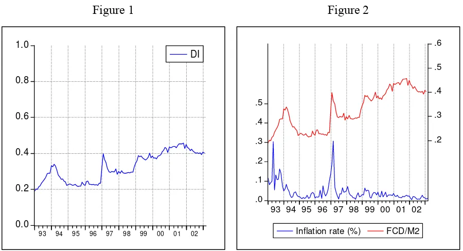
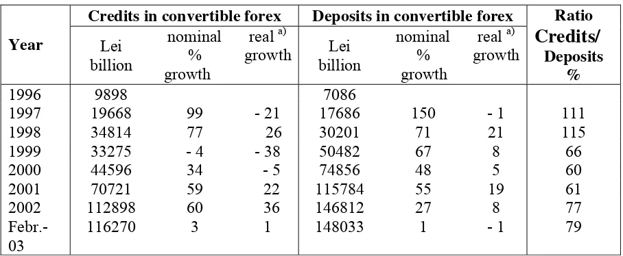
(i) We determined the ratio of foreign currency deposits in broad money (M2) for the period 1993:01-2003:03 in Figure 1. Using this indicator – which doesn’t measure only the foreign currency used for transaction purposes but also deposits used as a store of value –it is obvious that sharp increases in this proxy indicator for “dollarization” (IMF) correspond with episodes with high inflation.

[image:8.595.86.536.488.732.2]

A representation of this indicator together with the monthly rate of inflation is presented in Figure 2.

Figure 1 Figure 2

0.0 0.2 0.4 0.6 0.8 1.0

93 94 95 96 97 98 99 00 01 02

DI

.0 .1 .2 .3 .4 .5

.2 .3 .4 .5 .6

93 94 95 96 97 98 99 00 01 02

Inflation rate (%) FCD/M2

(9)

The two episodes with high inflation are in 1993 and 1997. Both periods are characterized by price liberalizations, fiscal reforms and stabilization programs. In 1997 the exchange rate was liberalized (from a system with an official exchange rate). It should be mentioned that Romania has experienced an exchange rate of full surrender system in early ’90 – its existence creates in some view incentives for currency substitution.

Also both (’93, ’97) were post-election years, so corrections to previously repressed administered prices were badly needed.

Although the proportion of foreign denominated deposits is large (around 40%) we should also note that the proportion of foreign trade in GDP is also increasing (with around 16-18 % points increase in the last 13 years).

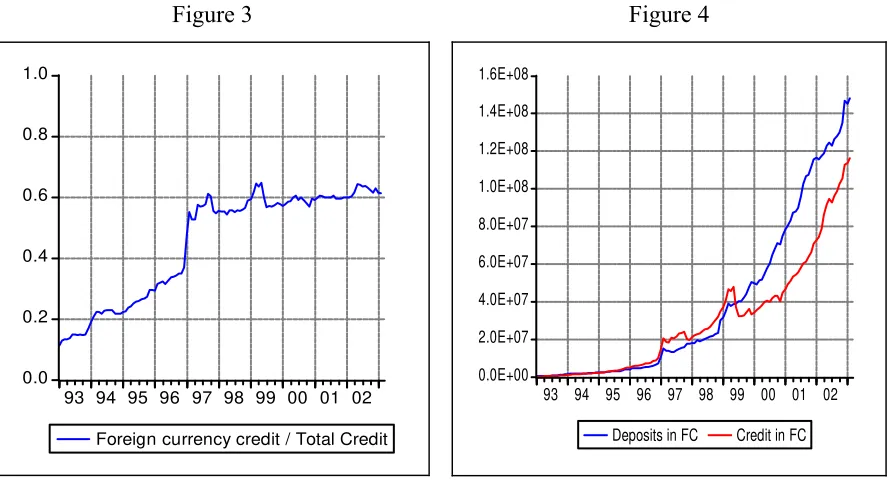
An analysis of commercial banks’ aggregate monetary balances reveals that in the last years banks have changed several times their behavior concerning forex intermediation. The ratio between domestic forex credits and forex deposits (Table 1) was above unit in 1997 and 1998, but worsened thereafter, reaching a minimum in 2000. Eventually the situation improved somewhat, but not enough to reach again supra-unitary ratios (normal, under the hypothesis of credit multiplying). The explanation for the sub-unitary ratio resides in commercial banks’ tendency, evident in 1999 – 2001, to place abroad large amounts of foreign exchange, despite lower yields, but with a much lesser risk. It should be recalled that those were the years when the restructuring of BANCOREX and of “Banca Agricola” took place, as well as a number of bankruptcies of smaller banks, which considerably increased the risk attached to Romanian assets. The ratio between external assets in forex and external liabilities in forex, rising sharply in 1999 – 2001, confirms the above. Starting 2002 commercial banks seem to have regained their trust in Romanian economy, reducing their external assets in forex (by 34 percent in real terms) and extending more internal credit in forex (by 36 percent in real terms).

(10)

[image:10.595.84.538.184.371.2]

crediting rules, because data for the first two months of 2003 show an increase of only 1 percent (in real terms) of forex credit.

Table 1

Credits in convertible forex Deposits in convertible forex

Year Lei billion

nominal % growth

real a)

growth Lei billion

nominal % growth

real a) growth

Ratio

Credits/

Deposits %

1996 9898 7086

1997 19668 99 - 21 17686 150 - 1 111

1998 34814 77 26 30201 71 21 115

1999 33275 - 4 - 38 50482 67 8 66

2000 44596 34 - 5 74856 48 5 60

2001 70721 59 22 115784 55 19 61

2002 112898 60 36 146812 27 8 77

Febr.-03

116270 3 1 148033 1 - 1 79

a) deflated by CPI

Source: NBR database

Actually, there is quite a lot a central bank can do in order to influence the composition of credit by currencies. After 1998, the National Bank of Romania has used quite actively the reserve requirements (RR) as a second – best option to sterilize important forex inflows, from the position of a net debtor to the banking system. Since November 1999, the rate of RR was made higher for Lei deposits (25%, then 30%) than for forex deposits (20%). As a result, credits in forex grew much faster than credits in Lei in 2000, 2001 and 2002, until the rates have been unified again, at 22%. After November 2002, the rate of RR was set higher for forex deposits (25%) than for Lei deposits (18%), with a view to effectively discourage further dollarization of the credit (the latter being inversely proportional to the rate of RR).

(11)

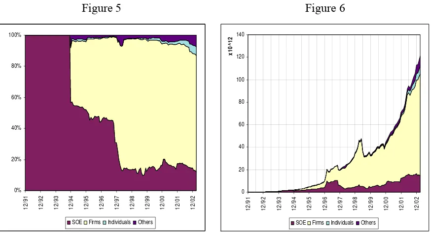
versus the DI, in absolute measures (as they are in Figure 4) they appear to be highly correlated.

The high level of this indicator is not surprising, and is anticipated in emerging economies, for example by Calvo (1999). Reasons for this high level of borrowing in foreign currencies could be institutional and informational.

The institutional cause of a high level of indebtness in foreign currencies could be legal requirements for a correlation between deposits and credits in foreign currencies.

As most of the banking sector is privatized, foreign banks which are the main supplier of loans have a natural tendency to denominate this in their currency. Also deficits (like current account deficits) will make that county dependent upon foreign savings.

Figure 4 indicates that except for roughly two years, the lending in foreign currencies has a bigger equivalent on the liabilities side – deposits in foreign currencies.

A decorrelation between these two would generate vulnerability because a sharp devaluation of the domestic currency would generate a systemic credit risk.

(12)

[image:12.595.90.535.77.317.2]

Figure 3

0.0 0.2 0.4 0.6 0.8 1.0

93 94 95 96 97 98 99 00 01 02

Foreign currency credit / Total Credit

Figure 4

0.0E+00 2.0E+07 4.0E+07 6.0E+07 8.0E+07 1.0E+08 1.2E+08 1.4E+08 1.6E+08

93 94 95 96 97 98 99 00 01 02

Deposits in FC Credit in FC

(13)

[image:13.595.85.532.119.317.2]

Table 2

External assets in convertible forex

External liabilities in convertible forex Year Lei billion nominal % growth

real a)

growth Lei billion

nominal % growth

real a) growth Ratio Ext. Assets/ Ext. Liabilities

1996 6544 4949

1997 13547 107 - 17 9103 84 - 27 149

1998 17289 27 - 9 8771 - 4 - 31 197

1999 22843 32 - 15 11131 27 - 18 205

2000 40100 76 25 13113 18 - 16 306

2001 50931 27 - 3 20651 57 21 247

2002 39881 - 22 - 34 33447 62 37 119

Febr.-03

38166 - 4 - 6 36791 10 8 104

a) deflated by CPI

The structure of foreign currency credit (Figure 5 and Figure 6) reveals that the main recipients were private firms. State owned enterprises (SOE) gradually loose their importance, as the privatization and restructuring process takes pace. Individual loans are in a rapid growth, especially mortgage and consumer credit.

Figure 5 0% 20% 40% 60% 80% 100% 12/ 91 12/ 92 12/ 93 12/ 94 12/ 95 12/ 96 12/ 97 12/ 98 12/ 99 12/ 00 12/ 01 12/ 02

SOE Firms Individuals Others

Figure 6 0 20 40 60 80 100 120 140 12 /91 12 /92 12 /93 12 /94 12 /95 12 /96 12 /97 12 /98 12 /99 12 /00 12 /01 12 /02 x 10^ 12

SOE Firms Individuals Others

[image:13.595.94.531.471.708.2]

(14)

As for other forms of financing for firms using foreign denominated currencies – as issuing shares and bonds – they aren’t significant as Romanian companies didn’t experience favorable conditions on foreign capital markets. Also investments abroad by Romanian individuals and firms are almost non existent, since capital account liberalization is an ongoing process and it will take some time before its effects can be felt.

Currency substitution in Romania is a topic in studies regarding the subject, and in some of them the authors are using data witch is not available (US Customs data – CMIR, FED data regarding inflows and outflows of dollars from US). These studies (Feige, 2002) estimate a

comprehensive dollarization index of 50.7% for Romania in 2001 (estimating the level of foreign currency in circulation) compared with 42.8% - the figure obtained using only the level of deposits in other currencies. This study also concludes that the correlation coefficient between the two measures is 0.994 for the period 1990-2001.

Another study (van Aarle, Budina, 1995) which uses a demand for money approach in evaluating currency substitution – and the econometric technique used being ECM – concludes that currency substitution seems important for the case of Romania.

The conclusion of the above is that currency substitution is more costly in an inflationary environment, in terms of perverse effects upon the role of forex as an unit of account, a medium of exchange and a store of value. Many of these costs could have been minimized, given a lower inflation. However, one must take into account that the National Bank of Romania was never given a strong mandate to fight inflation. Quite on the opposite, in an economy where the social and political concerns have been prevalent, the NBR found itself constrained to adopt “second – best” options and to muddle through, adopting a gradual disinflation process, albeit with higher economic costs.

(15)

(ii) There are several types of models used to investigate currency substitution. A review of the theoretical and empirical literature is realized by Giovannini and Turtleboom (1992). They identify three main types of models, but there are models which do not fit any of the categories.

The first category is comprised of models in which demand functions for domestic and foreign money are part of a static portfolio balance model, where optimal holdings of domestic and foreign assets are chosen together with currencies. Giovannini and Turtleboom state that this category of models treats domestic and foreign interest rates, together with exchange rates, as jointly determined, in a general financial equilibrium.

The second category includes models in which currency substitutability is estimated in narrower setup. In these models agents first decide on the optimal mix of monetary and non-monetary assets. In the second stage they decide how to allocate the monetary assets between the currencies in their portfolio based on the degree to which both currencies contribute to delivering money services and on relative opportunity cost between the two currencies.

The models in the third group usually start from the first order condition of representative agent’s dynamic optimization problem and, with some auxiliary assumptions, recover the parameters of interest, which allow the estimation of the substitutability of different currencies.

One type of models used to asses the importance of currency substitution is based on the theory of portfolio balance. These types of models assume that agents maximize the return to their wealth subject to a given level of risk. Agents can hold four types of assets and can switch between them simultaneously - Branson and Henderson (1985). These assets are: domestic money, domestic bonds, foreign money and foreign bonds. Usually the demand for these assets is specified and an explicit solution is obtained.

The first equation is a demand for local currency having as exogenous factors domestic and foreign (expected) interest rates, the expected exchange rate, domestic output, prices and wealth.

(16)

The third and fourth equations comprise models for the domestic and foreign bond demand of the domestic agents.

An important problem is linked with the capital mobility restrictions in place until recently in Romania, which prevented domestic agents from investing abroad. This type of restriction coupled with a rather shallow domestic bond market – in which major players are the commercial banks – make us exclude these equations from the estimation.

Also the second equation (the demand for foreign currency) is plagued with problems generated by the lack of data regarding the demand for foreign currency cash.

Empirical estimation of money demand functions is based on the transaction and/or portfolio theories. The transaction theories view money as a medium of exchange and demanded as an inventory for transaction purposes. Portfolio theories consider the demand for money as a part of the problem of allocating wealth among portfolio assets, which includes money. These portfolio theories emphasize store of value function for money.

A comprehensive literature review regarding the demand for money estimation – especially using error correction models (ECM) – is comprised in Sriram (1999). In this study theoretical problems are addressed, but also technical issues as the choice of money stock definitions, the choice of variable of scale and variables for opportunity cost of holding money.

Using this framework we estimated a demand for money equation for Romania.

The sample used is from 1997:06-2003:03. We did choose this sample to avoid the start of 1997 which was the moment of full liberalization of the exchange rate. The first six months of 1997 would have contained (probably) a structural break point in the data. Also the exchange rate liberalization could have introduced a shift in the demand for money in the same period.

(17)

CPI), logarithm of industrial production index – as a scale variable, the industrial production index is used as a proxy for the wealth or economic activity.

For the cost of opportunity we used: deposit interest rate for non-bank clients, the rate of change in the exchange rate (which approximates the expected change in the exchange rate and which captures the return of holding foreign currencies – EUR and USD, the basket of currencies is comprised of 60% EUR and 40% USD – which is roughly the structure of the foreign trade), the inflation rate as a proxy for the expected inflation rate – which was necessary because in economies with very narrow financial markets real assets can provide protection against inflation and are an alternative asset for non bank agents.

Usually a demand for money equation includes a T-bill rate (as a return on assets outside broad money), but in Romania’s case the data is discontinuous, and the T-bill market is very shallow. So we discarded this variable from the model. Also we should have used the expected depreciation rate corrected with the foreign interest variable, but in most of the period of our sample (1997:06-2003:03) capital mobility hasn’t been in place in Romania.

The estimation of a demand for money model is realized in a number of steps. The first is to asses the stationary properties of the series. ADF (Augmented Dickey Fuller) and PP (Philips Peron) test have been used. Also we used KPSS test (Kwiatkowski, Phillips, Schmidt, and Shin). We started testing for two roots and if two roots were rejected then we tested for just one root.

All variables included in the VEC are I(1). In some cases (inflation rate, the rate of change in the exchange rate) the three tests used have produced different results, so this variables could be also I(0). Even if these variables are I(0) they shouldn’t be excluded from the cointegrating vector (Dickey and Rossana (1994), Harris (1995)).

(18)

The results from testing the cointegration using the Johansen procedure had the following results:

Sample(adjusted): 1997:06 2003:02

Included observations: 69 after adjusting endpoints

Trend assumption: Linear deterministic trend

Series: LNM2ROL_R LN_I_IPI CSLCOSDMD CPL_IPCT_T DPM

Lags interval (in first differences): 1 to 2

Unrestricted Cointegration Rank Test

Hypothesized Trace 5 Percent 1 Percent

No. of CE(s) Eigenvalue Statistic Critical Value Critical Value

None ** 0.538342 100.4547 68.52 76.07

At most 1 0.263063 47.12237 47.21 54.46

At most 2 0.187988 26.05994 29.68 35.65

At most 3 0.137327 11.69139 15.41 20.04

At most 4 0.021486 1.498714 3.76 6.65

*(**) denotes rejection of the hypothesis at the 5%(1%) level

Trace test indicates 1 cointegrating equation(s) at both 5% and 1% levels

Hypothesized Max-Eigen 5 Percent 1 Percent

No. of CE(s) Eigenvalue Statistic Critical Value Critical Value

None ** 0.538342 53.33230 33.46 38.77

At most 1 0.263063 21.06243 27.07 32.24

At most 2 0.187988 14.36855 20.97 25.52

At most 3 0.137327 10.19268 14.07 18.63

At most 4 0.021486 1.498714 3.76 6.65

*(**) denotes rejection of the hypothesis at the 5%(1%) level

(19)

Unrestricted Cointegrating Coefficients (normalized by b'*S11*b=I):

LNM2ROL_R LN_I_IPI CSLCOSDMD CPL_IPCT_T DPM

-1.736722 3.331148 -2.646927 -11.12605 9.000816

1.337357 -14.69757 -3.145563 4.752014 -7.496296

-2.485940 6.042998 -4.491963 2.231383 4.717776

0.422647 0.735044 0.483318 2.799695 -10.99436

-12.80343 3.978027 1.340742 -1.194773 2.846529

Unrestricted Adjustment Coefficients (alpha):

D(LNM2ROL_R) 0.009142 -0.010561 0.009358 0.009174 -0.000420

D(LN_I_IPI) 0.017208 0.025121 -0.010443 0.000457 0.002479

D(CSLCOSDMD) 0.092988 0.018007 0.020910 -0.026812 -0.017417

D(CPL_IPCT_T) 0.045042 -0.022855 -0.045524 -0.022343 -0.002500

D(DPM) 0.000654 0.001375 -0.005158 0.005284 -0.002730

1 Cointegrating Equation(s): Log likelihood 468.1442

Normalized cointegrating coefficients (std.err. in parentheses)

LNM2ROL_R LN_I_IPI CSLCOSDMD CPL_IPCT_T DPM

1.000000 -1.918066 1.524094 6.406347 -5.182646

(1.07716) (0.44073) (0.87348) (1.12397)

We constructed the VEC model and tested its residuals for autocorrelation and serial correlation using the Portmanteau test and the LM test. We haven’t been able to reject the null hypothesis of no autocorrelation and no serial correlation at any lag.

The long run relationship is:

LNM2ROL_R = LN_I_IPI CSLCOSDMD DPM CPL_IPCT_T C

Coefficient 1.918066 -1.524094 5.182646 -6.406347 +13.04868 Std. Error (1.07716) (0.44073) (1.12397) (0.87348)

(20)

The sign of the industrial production index is the correct one, but the size of the coefficient is large (the quantitative theory of money indicates a value close to unity). The large elasticity of the output could be due to several reasons: omission of some important variables from the money demand equation (like inter firm arrears which constitute a substitute for money - generated by soft budgetary constrains), or the reason could be that industrial production index is not a perfect proxy for the GDP. To test if the coefficient is 1 we could impose a restriction assuming that B(1,1)=1 and B(1,2)=-1, this will yield a Χ2(1) of 0.4472 and an associated probability of 0.5036, so we cannot reject the hypothesis of a coefficient equal with 1.

The log run relationship with the restriction becomes:

LNM2ROL_R = LN_I_IPI CSLCOSDMD DPM CPL_IPCT_T C

Coefficient 1.000000 -1.411924 4.208897 -5.420551 12.56088

Std. Error (0.3852) (0.8347) (0.7035)

t-Statistic [3.6654] [-5.0420] [7.7047]

The speed of the adjustment coefficient (monthly change to the long run equilibrium) changes from -1.5876% to -1.5617% (Ericsson and Sharma have obtained for Greece a speed of adjustment coefficient of -8.1% - quarterly change towards the long run equilibrium; also they report several speed of adjustment coefficients determined on econometric studies on different European countries – for example - 9.3% for United Kingdom, - 15% for Germany, - 20% for France, - 26% for Netherlands).

The exchange rate depreciation coefficient has the correct sign (-) and the coefficient is close to that obtained by other studies carried out in the region for example Civcir (2003) – in a study on money demand in Turkey has a semi – elasticity of 1.4610.

(21)

The average deposit rate and the inflation rate have also the expected signs (+ and – respectively) and as the size they are also comparable with coefficient obtained in transition economies (for inflation Cuthbertson and Bredin (2001) did find for the Czech economy a coefficient of 4.04 and Ericsson and Sharma (1996) did obtain for Greece a coefficient of -3.38 for inflation and in their paper they quote studies (Taylor (1986)) in which the coefficients for the annual inflation are - 0.91 for Netherlands, - 2.67 for Germany, - 0.42 for France; as for the coefficient of the average deposit rate Ericsson and Sharma (1996) have a coefficient of 7.65 for Greece). These two coefficients clearly reveal that the interest rate on domestic assets is important in determining investment decisions, and the inflation rate elasticity demonstrates that an increase in inflation generates a fall in the demand for money.

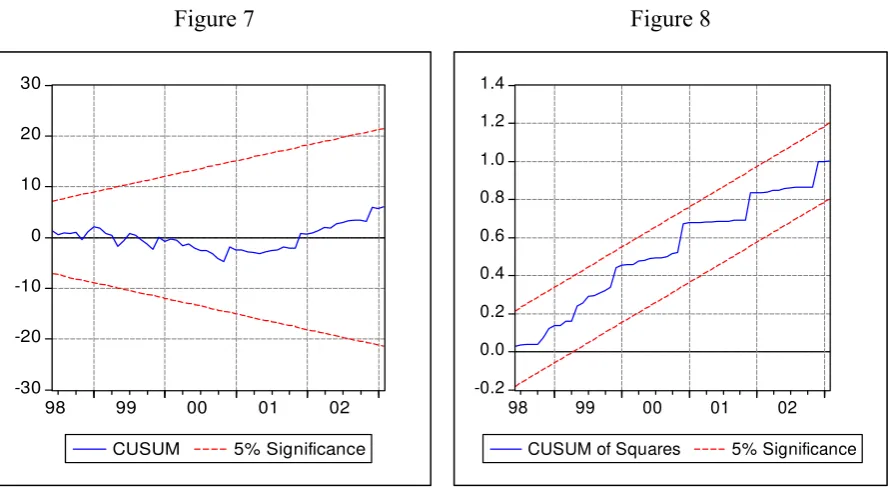
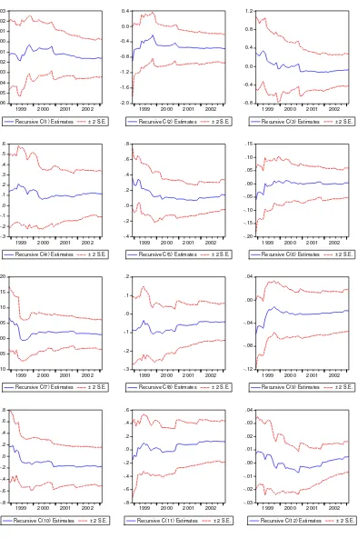
Parameter constancy is an additional and crucial issue to ensure a well specified equation. Parameter instability can be caused by financial crises or a shift in the demand for money. In order to asses the parameter stability the cointegrating equation is redone by using recursive estimation method. On the residuals from this equation we conduct several tests: CUSUM test (Figure 7), CUSUM of squares test (Figure 8) and recursive coefficient test ( Figure 9).

Figure 7 Figure 8

-30 -20 -10 0 10 20 30

98 99 00 01 02

CUSUM 5% Significance

-0.2 0.0 0.2 0.4 0.6 0.8 1.0 1.2 1.4

98 99 00 01 02

[image:21.595.89.534.477.721.2]

(22)

For the CUSUM test we cannot reject the hypothesis of constancy in parameters. Also the CUSUM of squares residuals indicate that we cannot reject the hypothesis of constancy ion parameters and volatility. The recursive coefficients test we can se the evolution of the coefficient as more and more of the sample date is used in estimation. For most of the parameters the estimation shows that they are stable.

(23)

[image:23.595.115.509.119.711.2]

Figure 9 -.06 -.05 -.04 -.03 -.02 -.01 .00 .01 .02 .03

1999 2000 2001 2002 Recursive C(1) Estimates ± 2 S.E.

-2.0 -1.6 -1.2 -0.8 -0.4 0.0 0.4

-0.8 -0.4 0.0 0.4 0.8 1.2

-.3 -.2 -.1 .0 .1 .2 .3 .4 .5 .6

-.4 -.2 .0 .2 .4 .6 .8

-.20 -.15 -.10 -.05 .00 .05 .10 .15

-.10 -.05 .00 .05 .10 .15 .20

-.3 -.2 -.1 .0 .1 .2

-.12 -.08 -.04 .00 .04

-.8 -.6 -.4 -.2 .0 .2 .4 .6 .8

-.8 -.6 -.4 -.2 .0 .2 .4 .6

-.03 -.02 -.01 .00 .01 .02 .03 .04

(24)

References

Berg, A. – Borensztein, E. (2000): “The Prons and Cons of Full Dollarization”, IMF Working Paper 50, 2000.

Calvo, G.A. (1999): “On Dollarization”, University of Maryland, 1999.

Civcir, I. (2003): “Broad Money Demand and Currency Substitution in Turkey”, The Journal of Developing Areas, Volume 36, Number 2, 2003.

Cuthbertson, K. – Bredin, D. (2001): “Money Demand in the Czech Republic since Transition”, Journal of Policy Reform, 2001.

De Freitas, M.L. (2000): “Dollarization hysteresis: further empirical evidence”,

Universidade de Alveiro, 2000.

De Freitas, M.L. (2001): “Revisiting the dollarization puzzle: Evidence from Bolivia, Turkey and Indonesia”, Universidade de Alveiro, 2001.

Dickey, D. A. - Rossana, R. J. (1994), “Cointegrated time series: A guide to estimation and hypothesis testing”, Oxford Bulletin of Economic and Statistics, 56 (3), 325-53. Doyle, B.M. (2000): “Here, Dollars, Dollars … Estimating Currency Demand and

Worldwide Currency Substitution”, International Finance Discussion Papers 657. Washington: Board of Governors of the Federal Reserve System, 2000.

Enders, W. (2000): “Applied econometric time series”, Iowa State University, John Wiley & Sons, Inc.

Ericsson, N. R. – Sharma, S. (1996), “Broad Money Demand and Financial Liberalization in Greece”, Board of Governors of the Federal Reserve System, International Finance Discussion Paper no. 559, 1996.

Feige, E. L. – Sosic, V. – Faulend, M. – Sonje, V. (2000): “Currency substitution, Unofficial Dollarization, and Estimates of Foreign Currency held abroad: the case of Croatia”, in Blejer, M. and Skreb M.: “Financial Policies in Emerging Markets”, Cambridge, Mass: The MIT Press.

(25)

Giovannini, A. – Turtelboom, B. (1992): “Currency substitution”, National Bureau of Economic Research Working Paper Series, No 4232, Cambridge 1992.

Greene, W. (1993): “Econometric Analysis”, second edition, Macmillan Publishing Company, New York.

Hamilton, D. J. (1994), “Time series analysis”, Princeton University Press.

Harris, R.I.D. (1995), “Using Cointegration analysis in Econometric Modeling”, Prentice Hall, 1995.

Komarek, L. – Melecky, M. (2001): “Currency substitution in the transition economy: a case of the Czech Republic 1993-2001”, Warwick Economic Research Papers, No 613.

Mongardini, J. – Mueller, J. (1999): “Rachet Effects in Currency Substitution: An Application to the Kyrgyz Republic”, IMF Working Paper 102, 1999.

Murray J. – Powell J. (2002): “Dollarization in Canada”, Bank of Canada, 2002

Nilsen, H. – Tullio, G. – Wolters, J. (2001): ”Currency Substitution and the Stability of the Italian Demand for Money before the Entry into the Monetary Union, 1972-1998”, Humboldt Universitat zu Berlin - Quantifikation und Simulation Okonomischer Prozesse 00-66.

Sonje, V. (2002): “The Impact of Currency Substitution on the Choice of Exchange Rate Regime: Lessons for UE Accession Countries”, International Center of Economic Growth, 2002.

Sriram, S.S. (1999): “Survey of Literature on Demand for Money: Theoretical and Empirical Work with Special Reference to Error-Correction Models”, IMF Working Paper no 64, 1999.

Uribe, M. (1997): “Hysteresis in a simple model of currency substitution”, Journal of Monetary Economics, No 40 185-202, 1997.

Van Aarle, B. – Budina, N.(1995): “Currency Substitution in Eastern Europe”, Tilburg University Discussion Paper, No 2, 1995.

Currency substitution in Romania

Munich Personal RePEc Archive