Computational Model for Agricultural Decision
Support System
Aditya Kumar Gupta
Sai Nath University Ranchi , India
Bireshwar Dass Mazumdar
School of Management Sciences Varanasi , India
ABSTRACT
Agriculture is one of the most important inventions of human civilization. The development of human civilization and development of agriculture technology were the two wheels of the cart. Unfortunately, it has been witnessed that the development of agriculture technology is not in the same ratio as human civilization is developed. Traditional tools and techniques used for forming are neither sufficient to predict nor, to optimize production results of yield. The agricultural data is diversified, complex and non-standard and information available about agriculture is in the form of static maps or tables or reports. Such information is not flexible enough to provide quick answers to the queries of farmers and decision makers. In this view the computerization of agricultural data is increasing need for economist and decision makers.
Data warehouse technology is a dynamic and versatile technology capable of providing information to farmers for efficient planning and implementation. Historically, data warehouses have been implemented in marketing and financial institutions. However, a remarkable shift in agricultural practices has occurred over the past century in response to new technologies. This also led to design an agriculture data warehouse and provide a decision support system, based on OLAP and data mining techniques. In the absence of computational model, an enormous amount of redundancy of data is observed, it increases complexities in OLAP. To overcome this redundancy in operational data, a mathematical procedure is needed for computation of decision coefficient. In this manuscript, we are introducing a computational model to optimize cropping system that leads to design of data warehouse for agriculture.
Keywords
Agriculture Technology, Data Warehouse, Computational Model, Decision Support System
1.
INTRODUCTION
Agricultural data is diversified and complex. It has large volume and many inter-related attributes. Extracting useful information and, decision making on this large volume of data is difficult and costly. As a result we require an efficient model that stores agricultural data in proper manner and efficient to response ad-hoc queries of the farmers and economist. In particular, agriculture technology is dependent on the prediction about weather and diagnosis of fertilizers in soil, type of crop and environmental issues. Too precisely for particular crop, we have to select proper quantity of various minerals and fertilizers related to a particular soil [1]. Similarly, the other attributes related to environment and weather may be classified on the basis of cold, rain, humidity, heat and other issues. The optimal selections of all these attributes help us to predict the production of crop and diagnose all related agricultural issues. The proposed model
produces mathematical values of decision making coefficient for production of various types of crop, in a particular land type and in a particular environmental attributes. The mathematical equations and supported tables are included to rectify the purpose of the model.
2.
LITERATURE REVIEW
A decision support system (DSS) is a computer-based information system that supports business or organizational decision-making activities. Decision support systems can be either fully computerized or human based or a combination of both. The expert system is a computer system that emulates the decision-making ability of a human expert.
An expert system for use in land drainage decisions was designed to diagnose the causes of drainage problems in the command area of an irrigation system [2]. Factors such as water regime in the soil profile, presence of a cultivation pan or an impermeable layer below the topsoil etc., were considered. An expert system for crop variety selection was developed for winter wheat in Scotland [3]. The developed system was designed to consider soil characteristics, water availability and prevalence of diseases. An agricultural decision support system intends to help the farmers to make better decisions and provide useful advice, thus fills the knowledge gap between the expert and the user.
3. COMPUTATIONAL MODEL FOR
AGRICULTURAL DSS
In this model we attempts to explore eight types of soil, depends on combinatory percentage of various fertilizers. We also classify crops in twelve major classes and propose a classifier for weather based on calendar months. These attributes are well placed in the model that systematically evaluates performance of crops for a particular soil, weather and for other agricultural attributes. The major inputs of the model are described in the following sections.
3.1 Calendar Months
Every crop needs specific weather for the best result; therefore the success ratio of a particular crop is depended on its seeding time. In our mathematical model, we use 12 months calendar as a main classifier of weather [4], we hypothetically assume maximum yield of a crop is possible when it is sowing in suitable month of the calendar. Although, forecasting about weather is unpredicted and dependent to some factors such as cold, rain, humidity and heat.
3.2 Crop-Set
their seeding time. These crop-sets consists number of crops having similar weather and environmental needs [5]. These crops are highly related to a particular class, and every crop belongs to particular crop-set. Here, we are putting similar crops in a set. These crop sets may be identified by the name of major crop belongs to it.
3.3 Fertilizer-set
In a particular type of soil, there are various fertilizers and minerals. The impact of fertilizers on production of any crop is significantly measured. We can identify various types of soil based on combinatory ratio of these fertilizers. In our study we identified 8 major fertilizers that are naturally available in soil, for this study fertilizer-set FS is defined as:
FS = {Urea (U), Phosphorus (P), Iron (Fe), Nitrogen (N), Zinc (Z), Sulfur (S), Calcium (Ca), Potassium (K)}. Further on the basis of the ratio of above fertilizers presence in soil, we can identify other soil types. Following table displays classification of soil type depends on percentage of fertilizers in a soil. In this table we hypothetically demonstrate 8 different type of soil based on fertilizer-set FS, however for the generalization purpose we can identify n types of soil, depending on combinatory ratio of fertilizers-set FS. We can also identified other fertilizer-sets , that may has other elements as defined in the set FS i.e., for any fertilizer-set where FS ≠ {Urea (U), Phosphorus (P), Iron (Fe), Nitrogen (N), Zinc(Z), Sulfur (S), Calcium (Ca), Potassium (K)}. By this way we can generalize the fertilizer-set, which may change with geographical regions.
In the model, further we assign 8-unit weight to each type of soil; each unit of weight corresponds to 10 % availability of a particular fertilizer in any fertilizer- set. For example soil type S1 contains 20 % of Urea, 50 % of Nitrogen and 10% of Potassium (Table 3.1) and, rest 20 % includes other elements in soil. We are not included such 20 % in our study, assuming it is non-deterministic minerals, as soil has many other impurities in it.
3.4 Irrigation
Irrigation is an important factor that is also incorporated in our model; we have taken three possible states of irrigation; high irrigation, medium irrigation and low irrigation. We have assigned constant values to each of these levels of irrigation, for the computational purpose.
3.5 Seed Quality
With the development of biotechnology, researcher produces high quality of seeds; the production rate of any yield is certainly dependent on quality of seed. As we have done for irrigation, quality of seeds is also classified in three levels, high quality, medium quality and low quality. We also
assigned constant values to these levels of seed quality in our model.
4. DETAIL DESCRIPTION
In this model we introduce a crop cycle based on their starting time and required soil type. The five main attributes: (1) calendar months (2) crop-sets (3) soil-type (4) irrigation and (5) quality of seeds, are placed in from inner cycles to outer cycles respectively (figure 4.1) [6]. Further the model is horizontally dived into in twelve regions each corresponds to month of calendar. The detail description of the model is given as follows:
The 12 calendar months are main classifier of weather and placed at innermost cycle (cycle 1) in clockwise direction. Every calendar month is represented by its order in calendar year. For example January is numbered as 1; February is numbered as 2 and so on.
The crop set are identified by major crop belongs to that crop set, these crop set are represented by roman numbers in the model. The crops are placed at cycle 2 in anti-clockwise direction. Each crop set is placed corresponding to their starting month. In our study we have assumed standard starting month of crop-set I is December, and it is placed in month of December. In the same fashion crop-set XII is placed in month of January, crop-set XI is placed in February and so on i.e. the sum of month number and crop set is always 13.
Cycle 3 corresponds to a particular fertilizer set, and type of soil belongs to that fertilizer set. In our study we identified 8 major fertilizers that are naturally available in soil, further we assign 1 unit weight for every 10 % of availability of a particular fertilizer in a fertilizer set. By this way, total weight of each soil type is 8 units per section. It means we are measuring only 80% of soil in our study, rest 20% are ignored assuming as non-deterministic data.
The cycle 4 corresponds to irrigation factor. We have assign total 3 unit weight to irrigation for high value of irrigation, 2 unit weights for medium irrigation and for low irrigation weight is equal to 1 unit.
At outermost cycle, i.e. cycle 5 , we have assign total 3 unit weight for high quality of seed , 2 unit weight for medium quality of seed and for low quality of seed weight is equal to 1 unit.
4.1 Mathematical Procedure and Working
To demonstrate working of the model, first we consider ideal state of the model; by the ideal state we mean the state in which a particular crop gives best possible production. In other words, if a crop receives most favorable fertilizer- set , most favorable weather with best quality of seed and , also receives proper irrigation, it results best possible production of yield and it is said to be in ideal state. In figure 4.1 the model is in ideal state i.e. the crop-sets are inseminated in the proper calendar month and also receives most suitable fertilizers, irrigation and seed quality is high. Mathematically, if Cj is sequence of crop- set and Mk is the sequence of sowing
month for any crop-set, then weight of seeding month and crop-set is given as:
Mw = (M + C ) ……….(4.1)
Where:
Let, Fw is the total weight of fertilization factor and Iw, and Sw
is the weight of irrigation factors and seed-quality factor
respectively, then total weight Tw of any particular crop set for best result is given as:
Figure 4.1 Computational Model for Agricultural Decision Support System
Explanation Figure 4.1
S1 = Soil Type 1
S2 = Soil Type 2
Tw = Mw + Fw + Iw + Sw ………... (4.2)
Where:
Mw = Weight of seeding month for any crop set i.e. Mw
= (Mj + Ck ).
Fw = Weight of fertilization factor
Iw= Weight of irrigation factor Sw = Weight of seed-quality factor
4.1.1 Assigning the Weights
Observe the values of calendar month cycle and values of crop-set cycle, as the calendar month is kept in clock-wise direction and crop-set are taken place in anti-clock wise direction that resultant , the sum of both of these cycle values is always 13, i.e. Mw = (Mj + Ck )= 13. Further the total weight of fertilization factor in ideal
state is calculated by assuming that all the required fertilizers of any fertilizer –set are available in proper ratio for a particular soil-type. We have already assigned 1 unit weight for every 10 % of availability, of a particular fertilizer in the fertilizer set. Hence, the total weight of each soil-type is 8 units per section. Therefore the total weight Fw = 8 for ideal state of the model. In our model we assign total 3 units of weight for
irrigation factor Iw ,the value for irrigation factor Iw = 3 if the irrigation is high , irrigation factor Iw = 2 if
irrigation is medium and , irrigation factor Iw = 1 if irrigation is low.
Similarly, the weight of seed-quality Sw is also assign by 3 unit of total weight and the values of Sw = 3 for high
quality seed, Sw =2 for medium quality and Sw= 1 for low quality seeds.
From the above considerations, the total weight Tw for ideal state is given by equation (4.2)
Tw = Mw+ Fw + Iw + Sw
Tw = 13 + 8 + 3 + 3 = 27 ……….…………(4.3) Hypothetically, we assume the production of crop is 100% if model score all 27 units of total weight Tw
Let Ω is a multiplicative constant to calculate the value of each point in percent then Ω is be given as
Ω = 100 / 27 = 3.7037………... (4.4) Therefore, every unit of weight corresponds to 3.7037 percent of success of the crop.
For a particular case , Let Pmis the total points of months , that are obtained by adding the values of cycle 1 and cycle 2 , i.e. Pm = (Mj + Ck) , where Mj is the sequence of month and
Ck is the sequence of crop-set in a particular region.
Similarly, we assume Pf is total points of fertilizers earn in cycle 3, Pi is total points of irrigation factor earn in cycle 4,
and finally Ps is the total points of seed-quality earned in the outermost cycle. Then, Pm, Pf , Pi and Ps is calculated as
follows:
4.2 Points of Month (
P
m)
According to the model the sum of month-sequence and crop-set are measured together, for the ideal state total weight of months Mw = 13, and if d is the displacement from seeding month of any crop-set from the seeding month in ideal state of the model, then we have
Pm = Mw × Ω – (d × Ω) Pm = 13 × 3.7037 – (d × Ω) or
Pm = 48.1481 – (d × Ω)…… ……… (4.5)
In above equation displacement d is the number of moths between sowing month of any crop, and sowing month in ideal state. Observe the model, any crop belongs to crop-set 1 is should be started in the month of December for the ideal state, suppose it is inseminated in the month of January or November, then the displacement d is equal to 1, and if it is inseminated in the month of October or February the displacement is equal to 2, and so on. Reader may observe this by rotating crop-set cycle on the inner month- cycle, based on this logic displacement can be calculate by following algorithm.
4.2.1 Displacement Algorithm
Displacement ( Mj, Ck )[7]
// Mj is the sequence of calendar month. // Ck is the sequence of crop-set
// Pm is the total point of month i.e., Pm = Mj +Ck, // where //1 ≤ j ≤ 12 and 1 ≤ k ≤ 12.
// disp is a temporary variable for displacement of any //crop-//set from ideal state, d is the output
//Pm,d and, disp are declared as integer variables and
// Mw = 13 initialize.
{
Pm = Mj + Ck ;
if (Pm = = Mw) disp = 0 ; if (Pm < Mw ) disp = Pm –1; if (Pm > Mw ) disp = Pm – Tw ; if (disp ≤ 6){
d = disp ; }
else {
d = 12 – disp ; }
}
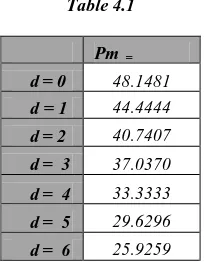
[image:4.595.378.480.527.658.2]With the above algorithm the value of d is between 0 and 6 i.e., 0 ≤ d ≤ 6. We now put d = (0,1,2,3,4,5,6 ) in equation (4.5) , then values of Pm are given as follows:
Table 4.1
Pm =
d= 0 48.1481
d = 1 44.4444
d= 2 40.7407
d= 3 37.0370
d= 4 33.3333
d= 5 29.6296
d= 6 25.9259
4.3 Point of Fertilization factor (
Pf
)
In section 4.1.1 , we have defined maximum weight of fertilization factor Fw = 8, i.e. Fw = (0,1,2,3,4,5,6,7,8) we can calculate point of fertilization factor Pf, by multiplying each
value of Fw by multiplicative constant Ω.
Pf = (Fw × Ω) ………..………...………..(4.6)
Table 4.2
Pf =
Fw = 0 0
Fw =1 3.7037
Fw =2 7.4074
Fw = 3 11.1111
Fw = 4 14.8148
Fw = 5 18.5185
Fw = 6 22.2222
Fw =7 25.9259
Fw =8 29.6296
4.4 Point of Irrigation factor (
Pi
)
From the section 4.1.1, possible values of irrigation factor Iw
is equal to 3,2 or 1 for high, medium and low irrigation respectively. Then irrigation factor Pi:
Pi = (Iw × Ω) ………..………...(4.7)
[image:5.595.113.222.540.636.2]For each possible value of Iw , Pi is given in following table
Table 4.3
Pi =
Iw = 1 3.7037
Iw = 2 7.4074
Iw = 3 11.1111
4.5 Point of Seed-quality factor (P
s)
Similarly, possible values of seed-quality factor Sw is equal to
3, 2 or 1 corresponds to high , medium and low quality of seed. Then seed-quality factor:
Ps = (Sw × Ω) ………..……….….(4.8)
For each possible value of Iw , Pi is given in following table
Table 4.4
Ps =
Sw = 1 3.7037
Sw = 2 7.4074
Sw = 3 11.1111
4.6 Calculating decision coefficient ‘α’
To calculate decision coefficient α for anyparticular case, first we calculate decision coefficient ‘αmax’ for ideal state, relook
the equation 4.2 and equation 4.3
Tw = Mw + Fw + Iw + Sw ………..……….(4.2) Tw = 13 + 8 + 3 + 3 = 27 ………..…... (4.3)
We now find decision coefficient ‘αmax’ for ideal state by
multiplying each coefficient of equation 4.3 with Ω
αmax = ( 13 + 8 + 3 + 3 ) × Ω
= 27 × Ω
= 27 × 3.7037 = 99.9999
For a particular case the value of success coefficient ‘α’, can be calculated by adding values of Pm, Pf , Pi and Ps i.e
α = Pm + Pf + Pi + Ps ………..………... (4.9)
5. EXPERIMENTAL RESULTS
We are including some experimental results for demonstration purpose of our model; the procedure of calculating success coefficient ‘α’ is also included for different cases. We have taken examples to simulate both of the major factors seeding time and, fertilization factors, further we have added some cases to visualize the affects of irrigation factor and seed quality facto. Consider following case that shows mathematical results regarding performance of crop.
5.1 Example (Case 1)
Let any crop of crop-set I, say - wheat is seeded in March beside its standard seeding month December in soil type 2 i.e. 20 % Urea , 30% Phosphorus, 10% Iron, 10% Nitrogen and 10% Zinc since the ideal soil type for crop-set is S2 therefore it gets maximum points of fertilizer factor, Fw = 8 . For the
simplicity it is also assumed that the quality of seed is up to the standard level and irrigation is up to the mark. Then Crop set is = I i.e. Ck = 1
Month Sequence is March i.e. Mj = 3
Then Pm = (Mj + Ck) = 3 + 1 = 4, from the algorithm 4.2.1 we find the value of displacement i.e. d = 3, however, more easily go through the table and you can find the same value of
d for the crop-set I in the month of November, putting d = 3
in equation 4.5 we get
Pm = 48.1481 – (3 × 3.7037) = 37.0370
As we have assumed that the availability of fertilizers in soil type is in ideal state, then points for fertilizer factor are maximum i.e. Fw = 8 since from equation 4.6 value of Pf Pf = 8 × 3.7037 = 29.6296
By the example the weights for irrigation Iw = 3 and seed quality Sw = 3, then from equation 4.7 and 4.8 , Pi = 11.1111 and Ps = 11.1111. We can calculate the value of success coefficient ‘α’ by equation 4.9 i.e,
α = 37.0370 + 29.6296 + 11.1111 +11.1111
= 88.8888 %
5.2 Example (Case 2)
Let any crop of crop-set I, say - wheat is seeded in January in soil type-4 i.e. 30% Phosphorus, , 20% Nitrogen 10 % Calcium and 20% Potassium, however from the model the ideal soli type for crop-set I is S2. Therefore points of fertilizer factor, Fw < 8. In this example we assume that the
quality of seed is medium level i.e. Sw = 2, but the value and irrigation factor is low Iw = 1. Then according to the model
Crop –set is = I i.e. Ck = 1
Month Sequence is January i.e. Mj = 1
Then Pm = (Mj + Ck) = 1 + 1 = 2, from the algorithm 4.2.1 we find the value of displacement i.e. d = 1, putting d = 1 in equation 4.5 we get
Ideal Land type for crop set I is S2 that has i.e. 20 % Urea, 30% Phosphorus, 10% Iron, 10% Nitrogen and 10% Zinc, in this case the crop is seeded in soil type S4 i.e. 30% Phosphorus, 20% Nitrogen 10 % Calcium and 20% Potassium. Then total point of fertilization may me calculated by finding the difference of fertilizers availability in S2 and S4.
Required Fertilizers (L2)=U2 + P3 + Fe1 + N1 + Z1
Available Fertilizers (L4) = 0 + P3 + 0 + N2 + 0 + Ca1 + K2
--- Total Points Fw = 0 + 3 + 0 + 1 + 0 + 0 + 0 = 4
---
Then from equation 4.6 value of Pf ,is gives as Pf = 4 × 3.7037 = 14.8148
By the example the weights for irrigation Iw = 1 and seed
quality Sw = 2, then from equation 4.7 and 4.8
Pi = 3.7037 and Ps = 7.4074. We can calculate the value of success coefficient ‘α’ by equation 4.9
α = 44.4444+ 14.8148 + 3.7037 +7.4074 = 70.3703 %
5.3 Example (Case 3)
For our third example we combining the situation of both of the above case and assuming the crop-set I, is seeded in month of March in the soil type 4. This time we consider the irrigation factor is up to the mark but seed quality is of medium quality. Then according to the model
Crop set is wheat i.e. Ck = 1
Month Sequence is March i.e. Mj = 3
Then Pm = (Mj + Ck) = 3 + 1 = 4, from the algorithm 4.2.1 we find the value of displacement i.e. d = 3, putting d = 3 in equation 4.5 we get
Pm = 48.1481 – (3 × 3.7037) = 37.0370
Again, total point of fertilization may me calculated by finding the difference of fertilizers in L2 and L4.
Required Fertilizers (L2) = U2 + P3 + Fe1 + N1 + Z1
Available Fertilizers (L4) = 0 + P3 + 0 + N2 + 0 + Ca1 + K2
---Total Points Fw = 0 + 3 + 0 + 1 + 0 + 0 + 0 = 4
--- Then from equation 4.6 value of Pf, is gives as
Pf = 4 × 3.7037 = 14.8148
This time the weights for irrigation Iw = 3 and seed quality Sw
= 2, then from equation 4.7 and 4.8
Pi = 11.1111 and Ps = 7.4074. We can calculate the value of success coefficient ‘α’ by equation 4.9
α = 37.0370 + 14.8148+ 11.1111 +7.4074
= 62.9629 %
6. CONCLUSION
The main contribution of the paper lies in the preparation of framework on agricultural data warehouse. The study includes identification and classifying of major agricultural attributes and places them in data warehouse schema. The model provides integrated information about whole crop cycle for the best results. We have also described some novel case of change such as starting time of crop, percentage of fertilizers
and impact of irrigation and seed quality. The model is supported by mathematical equations, and success percentage of crop in a particular weather and land type can easily be evaluated using these equations. This model may consider as a framework of agricultural decision support system and response to the ad-hoc queries of farmers using data mining techniques.
This paper may spurs cross-fertilization of ideas to relate data warehouse technology with agriculture sector. This may open new path for decision support cropping system. I will surprise if the model contribute or add some contribution in developing software application for agricultural data warehouse.
7. REFERENCES
[1] Anil Rai, Data warehouse and its Application in Agriculture.
[2] N. Haie and R.W. Irwin. 1988. Diagnostic expert systems for land drainage decisions. Irrig. Drain. Syst. 2(2): 139-146.
[3] O. W. Morgan, , M.J. McGregor, M. Richards and K.E. Oskouri. 1989. SELECT: An expert system shell for selecting amongst decision or management alternatives. Agric. Syst., 31: 97-110.
[4] Anil Rai , Sree Nilakanta and Kevin Scheibe, Indian Agricultural Data Warehouse Design , “Conference Managing Worldwide Operations & Communications with Information Technology”, 2007, Idea Group Inc
[5] M. R. Rao, Legumes Production in Traditional and Improved Cropping Systems in India.
[6] Aditya K Gupta, M.H. Khan, “Clock Based Model for Cropping System: A Frame work for Agricultural Data Warehouse”. National Conference, CSI, Delhi Chapter. Feb 2007.
[7] Horowitz, Sahni, Rajasekaran , “ Fundamentals of Computer Algorithms” Galgotia Publication, 2001.
[8] R. Kimball. The Data Warehouse Lifecycle Toolkit. J. Wiley & Sons, Inc. 1998
[9] Ramez Elmasri and Shamkant B. Navathe. Fundamentals of Database System, 3rd edition Addison Weseley, 2000. [10] Margaret H. Dunhan, Data Mining Introdouctry &
Advanced Topics. Pearson Education 2003.
[11] Alex Berson and Stephen J. Smith , Data Warehousing , Data Mining , and OLAP. Tata McGraw-Hill 2004. [12] Paulraj Ponniah , Data warehousing Fundamentals . J.