A Gradient Search Algorithm for the Maximal Visible Area Polygon Problem

http://dx.doi.org/10.4236/ajor.2015.53013

A Gradient Search Algorithm for the

Maximal Visible Area Polygon Problem

Helman I. Stern1_{, Moshe Zofi}1,2

1_{Department of Industrial Engineering and Management, Ben-Gurion University of the Negev, Beersheva,}

Israel

2_{Department of Industrial Management, Sapir College, Sderot, Israel}

Email: [email protected], [email protected]

Received 28 March 2015; accepted 8 May 2015; published 12 May 2015

Copyright © 2015 by authors and Scientific Research Publishing Inc.

This work is licensed under the Creative Commons Attribution International License (CC BY).

http://creativecommons.org/licenses/by/4.0/

Abstract

This paper provides a gradient search algorithm for finding the maximal visible area polygon (VAP) viewed by an interior point in a simple polygon P. The algorithm is based on a natural partition of P into convex sets, such that each element of the partition is associated with a unique analyt-ical form of the area function. We call this partition a back diagonal partition of P. Our maximal VAP algorithm converges in a finite number of steps, and is polynomial with a complexity of

(

2 2

)

O r n , for a simple polygon P with n vertices, and r reflex vertices. We use the maximal VAP

algorithm as a basis for a greedy heuristic for the well known guardhouse problemwith a compu-tation complexity of _{O r n}

( )

3 2 _.

Keywords

Maximal Visible Polygon, Gradient Search, Continuous Optimization, Guardhouse Problem

1. Introduction

A visual polygon is a polygon in which any pair of points is mutually visible. A visible polygon from a point x in a simple polygon P with n vertices can be found with a computational complexity of O n

( )

by the algo-rithm of El Gindy and Avis [1]. For each visible polygon, one may associate a real number representing its area. The area function over all points x P∈ is not well behaved, being in general neither convex nor concave, in-cluding points that may be not differentiable and even discontinuous. Some properties of polygonal area func-tions may be found in [2].

po-lygon. We denote this problem as the maximal visible area polygon (VAP) problem. This problem was studied by Cheong et al. [3], which suggested sampling a finite number of points inside the polygon found by its trian-gulation.

The algorithm we suggest for this problem is based on a gradient search which converges with a finite number of steps. In order to determine the size of each step taken in the gradient direction, we use a specialized partition of the polygon P into convex sets referred to as a back diagonal partition (BDP). This decomposition arises naturally through the introduction of “back diagonals” in such a manner that the area functional expression is invariant within the domain of each element of the partition. Gradient information along with jump points is combined in an algorithm which traces a path from some initial point in the polygon to a local maximal point. The developed algorithm has a computational complexity of _{O r n}

( )

2 3 _{for a polygon P with n vertices and}

r reflex vertices. Such a path may be used to guide a mobile search robot in an enclosed 2D area.

A related problem of placing the minimum number of stationary guards to visually cover a room represented as a 2D polygon was first presented by Klee in 1973 [4] as the art gallery or guardhouse problem. The objective was to find the smallest set of points in a polygon, such that every point inside the polygon would be visible to at least one point in the set. Two points are visible to each other, if the line of sight connecting them lies inside the polygon. Several heuristics and complexity calculations are provided in [5] and [6] for different extensions of the guardhouse problems in which the observers are restricted to the vertices of the polygon, and the edges of the polygon, or not restricted at all. In this paper, we offer a greedy algorithm, which repeatedly uses the gra-dient search method for finding the maximal VAP, and for solving the guardhouse problem. This greedy heuris-tic terminates after a finite number of steps and is polynomial with time complexity of _{O r n}

( )

3 2 _{. Although the}

original problem was described in terms of the positioning of guards, it had application to the positioning of surveillance cameras, motion sensors or other detection devices in enclosed environments. We assume that omni vision cameras (or several back to back cameras) are placed at the selected positions. This problem has recently become a popular security problem. For example, currently England has 5 million CCTV security cameras and is adding them at the rate of 100 per day in both inside and outside environments.

In Section 2, we define the maximal VAP problem and introduce useful notation. In Section 3, we introduce the concept of a hidden region, its area, and a back diagonal partition. These set the stage for the introduction of the maximal visible area polygon (VAP) gradient search algorithm described in Section 4.In Section 5, we use the gradient maximal VAP algorithm to form a basis for a greedy algorithm to solve an application in the form of the guardhouse problem, and illustrate it with a small example. Section 6 provides conclusions and future work.

2. Problem Definition and Notation

Before embarking on a formal definition of the problem we present a number of definitions and associated nota-tion. A polygon P is a closed plane figure bounded by at least three straight connected line segments. A poly-gon P containing n line segments can be described using the vertices along its boundary P=

{

v v1, , ,2 vn

}

.

Let ei denote a directed edge between adjacent vertices of P where ei=

(

v vi, i+1

)

, i=1, , n and n+ =1 1. A simple polygon is a polygon which does not contain any holes and whose edges do not intersect. Two points u and v in P are mutually visible if for all points w such that w=λu+ −

(

1 λ

)

v, λ∈

[ ]

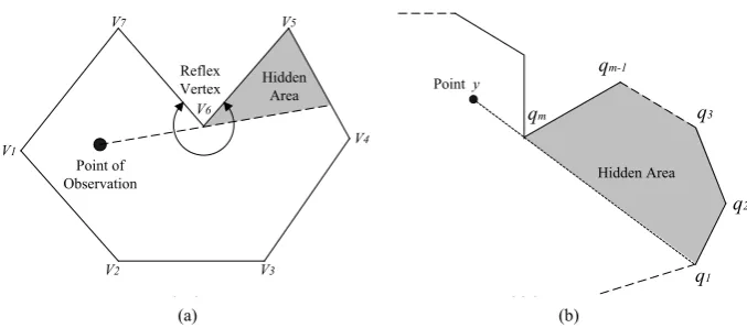
0,1 , lie within P. A vertex of P is said to be non-convex or reflexive if the angle between the two segments that share it as endpoints is greater than 180 _{when viewed from the interior ofP. Reflex vertices can create hidden areas} when viewed from some points inside the polygon. Figure 1(a) shows a simple polygon where vertex v6 is a reflex vertex, inducing a hidden area with respect to an observation point.

We define V p P

(

,

)

as a visibility polygon, such that each point in V is visible by an observation point p. The area of V is denoted as A V p P

(

(

,

)

)

. When understood these will be written simply as V p

( )

and

( )

A p . Given a polygon P of size n, and a point p inside P, the visible polygon V p P

(

,

)

and its area

(

)

(

,

)

A V p P can be determined with a time complexity of O n

( )

[1]. The Maximal VAP Problem

Define a maximal visible area polygon (VAP) problem as finding a point p∗ _{for which}

(

₍

₎

)

,

[image:3.595.128.467.81.230.2]

(a) (b)

Figure 1. Simple polygons with hidden areas. (a) A simple polygon containing a reflex vertex; (b) A region created by a chain of vertices which are not visible from an observation point.

(

)

(

)

(

(

)

)

Max , ,

p P A V p P A V p P

∗

∈ =

The expression for the signed area of a polygon P, with vertex coordinates

{

(

x y ii, i

)

, =1, , n

}

reduced modulo n y0= yn, yn+1=y1, is

( )

(

1 1

)

1 1 2

n

i i i

i

A P x y+ y−

=

=

∑

−

Note, that A P

( )

represents the signed area of the polygon P, i.e. A P

( )

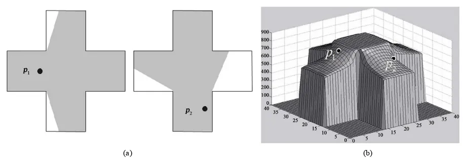
>0, if the vertices of P are in-dexed in counterclockwise order. The visible area function over all x P∈ is not well behaved, being in general neither convex nor concave. Moreover, it may contain points that are not only non differentiable but disconti-nuous. For the example in Figure 2(c), the top flat square has a non differentiable boundary and discontinuous drops at its corners.

3. Local Maximal Visible Area Polygon (VAP) Gradient Search Algorithm

We propose a gradient search method which starts with a given observation point, and moves it in the direction of the maximal gradient until a local maximum is achieved. At each step of the algorithm, a different visible area is calculated (i.e. the polygon minus the hidden regions) as a function of the current point. The result of a step in the maximal area gradient direction will give the

( )

x y, coordinates of the new observation point. Since there are several local gradients (one for each hidden region), the final direction is determined by the resultant vector. For example, if polygon P has two hidden regions with respect to a given point p , then two gradients are calculated (one for each hidden area). If the gradients for hidden regions I and II are

(

x y1, 1

)

and

(

x y2, 2

)

, re-spectively, then the final gradient

(

∇ ∇_x, _y

)

will be

(

x x y y1+ 2, 1+ 2

)

. Below we present several definitions, which will form the basis of a gradient search method to be described subsequently.

3.1. Basic Definitions and Notation

Given a simple polygon P=

{

v v1, , ,2 vn

}

with vertices ordered in counterclockwise order, for any three

consecutive vertices v1=

(

x y1, 1

)

, v2=

(

x y2, 2

)

, v3 =

(

x y3, 3

)

define a turn: T as:

(

3 2

)

(

2 1

)

(

3 2

)

(

2 1

)

T = y −y ⋅ x −x − x x− ⋅ y −y . We say that v v v1 2 3 is a left turn if T is positive, a right turn if T is negative, and not a turn otherwise.

Proposition 1 Let a chain Q be a sequence of connected, nonintersecting line segments. Given two points

y and z, such that the line segment yz does not intersect any line segment of Q, then y and z are said to be mutually visible with respect to chain Q.

Proposition 2 Let Q=

{

q q1, , ,2 qm

}

be a simple chain such that q1 and qm are visible with respect to

Q. If a point y is exterior to the region enclosed by

(

Q q, 1

)

and collinear with q1 and qm, then the region Hidden

Area

Hidden Area Point of

Observation V7

V1

V2 V3

V4

V5

V6

Reflex

Vertex Point y

q1 q2 q3 qm-1

qm

[image:4.595.83.540.80.238.2]

(a) (b)

Figure 2.A cross shaped polygon. (a) The visible polygon from point p1 (area = 93.6%); (b) The visible polygon from

point p2 (area = 82.9%); (c) The area function.

enclosed by

(

Q q, 1

)

is not visible from y. The proof appears in [1].

Figure 1(b) shows an example of a point y exterior to a chain Q=

{

q q1, , ,2 qm−1,qm

}

. The point y is

collinear with q1 and q5, and therefore, cannot see the region enclosed by

(

Q q, 1

)

. A line segment q q1 m is

said to be a window of y with respect to the region enclosed by

(

Q q, 1

)

. This region is said to be a hidden re-gion with respect to y. Note, that if qm is visible from y then so is q1. We denote the window,

(

1, m

)

W = q q of y, as a left hand window (LHW) if yq qm m−1 is a left turn, and as a right hand window (RHW) if yq qm m−1 is a right turn. Looking back at Figure 1, we can see that yq qm m−1 is a left turn. Let p be a viewpoint inside P and s a reflex vertex on the boundary of P. We classify reflex vertices as active or inactive according to the possibility of each creating an area occluded from p. In order to determine whether a reflex vertex s is active or inactive with respect to a given viewpoint p, we extend the adjacent edges of s into the interior of P until they hit the boundary to obtain back diagonals χ1 and χ2. If p and s are mutually visible and p lies outside the angle χ1, , s χ2, then s is said to be an active reflex point, otherwise s is inactive. Given a viewpoint p and an active reflex point s, define a ray Λps from p in the direction of s and passing through s. Let I =

{

p p1, , ,2 pq

}

be the set of intersection points of the ray with the

boundary of P, ordered according to the distance from p. Denote the intersection point closest to p as a reflection point p′_{. Figure 3(a) shows the reflection point p}′ _{(the first intersection point) with respect to a}

viewpoint p and an active reflex vertex s.

3.2 Back Diagonal Partition (BDP)

Consider a pair of vertices u and v on the boundary of P, such that u is a reflex vertex and v is visible from u. Define a diagonal uv as a line segment directed from vertex u to vertex v. A back diagonal uv′

with respect to uv is a line segment joining the vertex u and the point v′, where v′ is the nearest point on the edge of P visible in the reverse direction of uv. The point v′ is said to be a reflection point on the boundary of P visible from v along a ray directed from v through u. Figure 4 shows a back diagonal

uv′ created by a reflex vertex u and a vertex v visible from u.

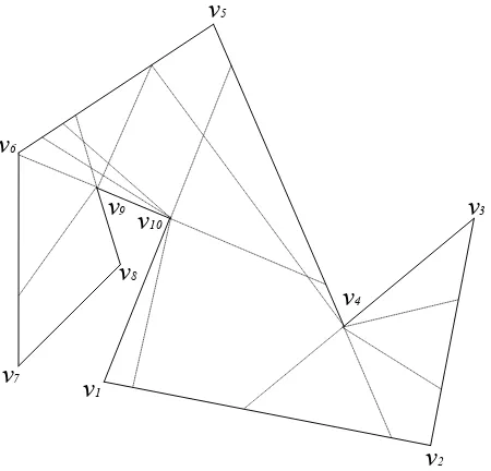
Figure 5 shows an example of all back diagonals (dotted lines) induced by the reflex vertices. The introduc-tion of all back diagonals induces a back diagonal partiintroduc-tion (BDP) of P. Such a partition is a planar graph de-fining a set of internal regions. Note that five back diagonals are induced by vertex v10-one for each of the ver-tices in P visible from v10.

Proposition 3 A BDP of P partitions P into a collection of regions, each a convex sub polygon of P.

Proposition 4 A back diagonal is an edge in a BDP such that viewpoints in the neighborhood on either side of it have different visible and area polygonal functional expressions. Thus, each region in a BDP has a unique visible and area polygonal functional expression.

[image:5.595.74.525.81.207.2]

(a) (b)

[image:5.595.231.374.247.337.2]

Figure 3. (a) A reflection point p′_{, with respect to a given viewpoint} p and an active reflex vertex s; (b) Left and right hand hidden regions with respect to a given viewpoint p.

Figure 4. A back diagonal uv′ created by a reflex vertex u and a vertex v visible from u.

Figure 5.A back diagonal partitioning for a polygon with three reflex vertices.

3.3. Hidden Regions

Note that the gray areas in Figure 3are hidden regions with respect to the viewpoints p. We define back edges for two cases. Case 1: If p′ _{is an interior point of an edge} e of P, then p′ _{is said to be a reflection point}

of p on e through the active reflex vertex s, and e is called a back edge of p through s. The edge 7 8

v v in Figure 3is the back edge of the viewpoint p through the reflex vertex s.Case 2: If p′ coincides with a vertex vi of P, then the back edge is taken as e=

(

v vi, i+1

)

. In this case, vi and s induce a back

diagonal on which p lies. For ease of exposition, all of the following will be in terms of case 1. Note, that case 1 corresponds to a point p that does not lie on a back diagonal with respect to s. A left hand hidden region

( )

H L with respect to p, a left hand active reflex vertex s, a reflection point p′ _{and its back edge v vi−1 i, is}

Viewpoint

v

6

v

9

v

2

v

3

v

4

v

5

s1

s2

v

7

v

8

v

1

p2'

p1' Hidden

Area Viewpoint

v

9

v

1

v

2

v

3

v

4

v

8

s

Reflex Vertex

Reflection point

v

5

v

6

v

7

Right hand hidden region

Left hand hidden region

p'

p p

u

v

v'

v

1

v

2

v

3

v

4

v

5

v

6

v

10

v

7

v

8

[image:5.595.188.413.366.582.2]

a region bounded by the polygon defined by the circular vertex list:

( )

(

, ,

)

(

, ,i i1, i 2, , , ,k

)

H L =H L p s = p v v v′ + + v s p′

where v v vi, i+1, i+2, , vk, and s are the original vertices of P in CCW order. A right hand hidden region

( )

H R is similarly defined for a right hand reflex vertex as H R

( )

=H R p s

(

, ,

)

=

(

p s v v v′, , ,i i+1, i+2, , , v pk ′

)

. Figure 3(b) provides an illustration of H L

( )

and H R

( )

for a given observation point p.

We can now define a visible polygon in terms of the definitions given above. Given a polygon P and an observation pointp, define the visible polygon V p

( )

as the polygon comprised of subsequences of the origi-nal vertices of P and all windowswith respect to p. The visible polygon V p

( )

contains all visible vertices and the reflection points of all active reflex vertices with respect to p. From proposition 2 it should be clear that the regions enclosed by H L

( )

and H R

( )

are not visible from p.

3.4. Calculation Formulas Using Hidden Areas

Define a rectangular coordinate system in _E2 _{such that each point i in E}2 _{is represented by a set of ordered} real valued coordinates

(

x yi, i

)

. Given the coordinates of an observation point p=

(

x yp, p

)

, the end points of

back edge

(

v v1, 2

)

, and an active reflex point s, the reflection point p′ can be calculated as a function of p and has the general form:

(

)

1 2 3 7 8 9

4 5 6 10 11 12

, p p , p p

p p

p p p p

x y x y

x y

x y x y

ρ ρ ρ ρ ρ ρ

ρ ρ ρ ρ ρ ρ

′ ′

 + + + + 

= _ _

+ + + +

 

Here, ρi

(

i=1, ,12

)

are constants in terms of the points v v1, 2 and s. The hidden area as a function of p′ _{(the reflection point) has the following form:}

( )

(

)

1 p 2 p 3,

(

( )

)

4 p 5 p 6

A H L =α x′+α y ′+α A H R =α x′+α y ′+α

Here, αi

(

i=1, ,6

)

are constants comprised of the coordinates of the original boundary vertices of P.

This is a direct result of applying Equation (2) to the boundary vertices

(

p v v v′, ,i i+1, i+2, , , , v s pk ′

)

,

(

p s v v v′, , ,i i+1, i+2, , , v pk ′

)

of the left and right hidden regions, respectively. Given a point p in P, asso-ciate with it a set of active reflex vertices. Let m pL

( )

and m pR

( )

represent the number of left and right

ref-lex vertices with respect to p. Each active reflex vertex i has an associated hidden region. Let

(

, ,

) (

, ,

)

H L p i H R p i represent a left/ right hidden regions of p associated with an active reflex vertex i, respectively.

The collection of left and right hand hidden regions associated with p are denoted as;

( )

{

(

, , ,

)

1,2, ,

( )

}

L L

S p = H L p i i= m p and S pR

( )

=

{

H R p i i

(

, , ,

)

=1,2, , m pR

( )

}

, respectively. Since

in-tersections of hidden regions are empty (except for possible vertex points), the area of the visible polygon may be represented as follows:

(

)

( )

( )

(

)

( )

(

)

1 1

, m pL , , m pR , ,

i i

A V p P A P A H L p i A H R p i

= =

 

= − +

      

  _

∑

 

∑

 _

This area function will be derived in terms of the rectangular

(

x yp, p

)

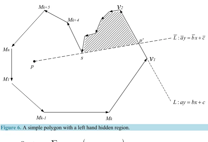
coordinates of point p, in order to

determine the directional move of p, such as to increase the visible area. For example, Figure 6 shows a poly-gon P=

{

M M1, 2, , M v vk, , , , ,1 2 s Mk+4,Mk+5, , Mn

}

, with a H L p s

(

, ,

)

, and a visible polygon

(

,

)

{

1, 2, , k, , , ,1 k 4, k 5, , n

}

V p P = M M M v p s M′ + M + M .

Let AL A P=

( )

−A H L p s

(

(

, ,

)

)

represent the area of the visible polygon associated with the view point p and a left hand hidden region H L p s

(

, ,

)

. Using

( )

2 and isolating the coordinates

(

x yp′, p′

)

we get the area in terms of p′_:

( )

(

( )1

)

(

( )1

)

[image:7.595.126.470.79.314.2]

Figure 6. A simple polygon with a left hand hidden region.

( )

(

( )1 ( )1

)

( )1 ( ) ( 4)

1, , , 4, ,

Const M i M i M i v M k s M k

i= k k+ nx y + y − x y x y +

=

∑

⋅ − − ⋅ + ⋅

The only relevant vertices are the reflex vertex s (which created the hidden region) and v1 which is the visible vertex of the edge e=

(

v v1, 2

)

, the back edge of p through s. Note that p′ is the intersection point between the line collinear with

( )

p s, and e. Repeating the process for a right hand side region, where v2 is the visible vertex of the back edge e we obtain:

( )

(

( )2

)

(

( )2

)

2AR p′ = yv −y xs ⋅ p′− xv −xs ⋅yp′+Const

The individual coordinates of p′ can be convex or concave, increasing or decreasing or constant in x_p and

p

y depending on the orientation of the ray ps and the back edge

(

v v1, 2

)

.

4. Gradient Search Algorithm for Maximal VAP

Following are the steps of a gradient search algorithm for finding alocal max to the maximal visible polygon problem. Given the current point p, the algorithm finds the maximal gradient direction and moves p until one of a number of events occurs. These events are determined when the functional form of the area function undergoes a change if the move is continued. This occurs, for example, when the point hits a back diagonal or an original edge of P. Also, when the refection point moves to an end point of its back edge, or when a new reflex point becomes active. At any of these events a new area function is introduced and the gradient is recalculated to determine a new movement direction.

4.1. Determination of the Maximal Gradient Direction

Since xp′ and yp′ depend on the view point p, we must rephrase the area’s formulation using its coordi-nates. To do this two lines are constructed: :L ay bx c= + (connecting p and s) and :L ay bx c= + (col-linear with the back edge

(

v v1, 2

)

) (see Figure 5). The intersection of L and L is the point

(

x yp′, p′

)

. The right side of (9) contains functions of p′.

(

x yp′, p′

)

ac ac_{ab ab}, _{ab ab}cb cb

 − − + 

= _{− + − +} 

 

( ) ( )

2 2

, s s , s s

P P

AL AL _b ay bx c _a ay bx c

x y ab ab ab ab

 

∂ ∂

 _{= ⋅} − −  _{− ⋅} − −  _

  _{     }

∂ ∂  − +   − + 

 _{ } 

p

v

1

s

v

2

p' Mk+4

Mk+5

Mn

M1

Mk

Mk-1

c x b y a

L: = +

c bx ay

( ) ( )

2 2

, s s , s s

p P

AR AR _b ay bx c _a ay bx c

x y ab ab ab ab

 

∂ ∂ _{= − ⋅}  − −  _⋅ − −  _

  _{   }

 _{∂ ∂}   _{ − +   − + } 

   

The total gradient ∇p is the sum of the partials for all active reflex vertices with respect to p.

(

)

( )

( )

( )

( )

( )

( )

( ) ( )

, ,

L R L R

p x y

s S p P s S p P s S p P s S p P

AL AR AL AR

x x y y

∈ ∈ ∈ ∈

 ∂ ∂ ∂ ∂ 

∇ = ∇ ∇ =_{ ∂} + _{∂ ∂} + _∂ _



∑

∑

∑

∑



where, S pL

( )

and S pR

( )

are all active left and right reflex vertices with respect to p, respectively.

4.2. Max VAP Algorithm (the Gradient Search Algorithm)

Although this algorithm is based on movements between sub regions of a BDP, there is no need to actually con-struct it. It is only necessary to concon-struct the back diagonals (line equations). This is because the algorithm searches for a critical event when the observer crosses a back diagonal. At his point, based on proposition 4, a recalculation of the area and new gradient are necessary.

The Steps of the Procedure

Given a simple polygon, and a point _p0 _{in P. Set p p=} 0_. Step 1 Compute the area of P as A P

( )

.

Step 2 Determine the visible polygon V p

( )

from p and its area A V p

(

( )

)

≤ A P

( )

. Identify all “active” reflex vertices s s1, , ,2 sw and the corresponding set of windows: W p

( )

=

{

Wk =

(

s p kk, k′

)

=1, , w

}

, where

k

s is the _kth _{active reflex vertex, and} k

p′ _{its reflection point which lies on the interior or endpoint its}

asso-ciated back edge eik = v vik, ik+1. If W p

( )

=φ, go to Step 7 (Stop).

Step 3 Find the total gradient ∇p that maximizes the increase in A V p

(

( )

)

, using (12) and Proposition 5. If

no such gradient exists, stop and go to Step 6.

Step 4 If p lies on an original edge of P, calculate a new gradient direction so as to slide along the edge in a direction such that the angle between the original gradient direction and the edge is minimal.

Step 5 Move p in the gradient direction until one of the following critical events occurs: a) p hits a vertex or edge of P.

b) One of the reflection points pk slides to the endpoint of its back edge eik (i.e. one of the vertices of P).

c) If one of the windows Wk becomes collinear with one of the edges that forms a reflex vertex, i.e.;

(

s sk, k−1

)

or

(

s sk, k+1

)

for a LH or RHwindow, respectively. This reflex vertex becomes inactive; drop its associated window from W p

( )

.

d) A new reflex vertex becomes active. Add the associated window to W p

( )

.

Step 6 If W ≠φ, compute the new point p, and return to Step 2; otherwise, W =φ, and the entire polygon is viewable from p.

Step 7 Stop. No local improvement is possible. Let p∗ _{be the best point. Compute A V p}

(

( )

∗

)

_{, the total}

visible area from p∗_.

Note that the events in Step 5 correspond to the intersection of the gradient direction vector and all back di-agonals.

Proposition 5 The sequence _{A V p}

(

( )

0

)

_{,A V p}

(

( )

1

)

_{, ,A V p}

(

( )

i

)

_{, ,A V p}

(

( )

∗

)

_

  is increasing in i.

Proposition 6 The Gradient Search Algorithm converges in a finite number of steps. This is true since the

sequence in Proposition 1 is bounded from above by the area of P.

Proposition 7 The gradient search algorithm has a time complexity _{O r n}

( )

2 2 _.

0

p and p∗ _{as back diagonals are not revisited. Thus, the total time complexity of the gradient search algo-}

rithm is _{O n}

( )

_{+ +}

[

_{r rn rn O r n}

]

_{⋅ ≈}

( )

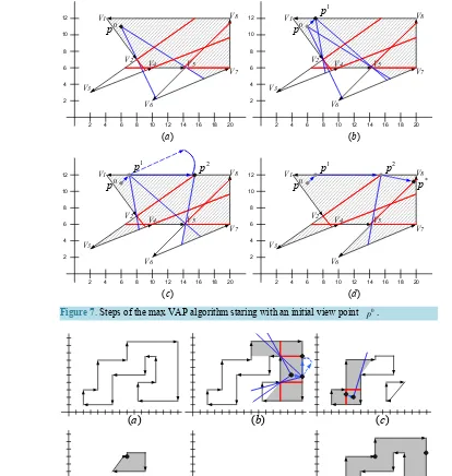
2 2 _.

4.3. Illustrative Example for the Maximal VAP Problem

The example in Figure 7provides a demonstration of the algorithm for the case of a simple polygon with three reflex vertices, one of them, v4 remaining inactive throughout. The sequence of points and visible areas are

0 1 2

p _→p _→p _→p∗_{, and A}0 _=86.5→A1_=87.0→A2 _=95.5→A∗ _=100.

5. Application-Solving the Guardhouse Problem

The guardhouse problem, proven to be NP-Hard in [4], is defined as the problem of the finding the minimal number of observation points F in a given a simple polygon P such that, the union of the visible area of all points in F equals P.

{

}

(

)

Min , , subject to : ,

p F

F F P V p P P

∈

⊆

_∪

=

A greedy algorithm is described for solving the guardhouse problem which repeatedly uses the maximal VAP algorithm. The idea is to start with a simple polygon, and remove a maximal VAP. This operation can result in disconnected components, each in itself a simple polygon. The process is repeated for any remaining compo-nents. Each removal results in an additional observation point, so that the number of removals equals the number of points needed to view the entire original polygon.

5.1. The Greedy Heuristic

Given a simple polygon P, let Π be a collection of polygons.

1) Initially set Π =

{ }

P , remove P from Π and set it to the current polygon P.

2) Start with a random point p in P. Call the Max VAP gradient search algorithm to find the point p∗_,

(

,

)

V p P∗ _{and A V p P}

(

(

∗_,

)

)

_.

3) Let P be the set of simple polygons obtained by subtracting the visibility polygon V p P

(

∗,

)

_{from P.} (i.e. the parts of the polygon P which are not visible from p∗_{). Add P to the collection of polygons Π.}

4) If Π =φ stop, otherwise;

5) Select a polygon P in Π and remove it, and return to Step 2.

The greedy heuristic described above terminates after a finite number of steps. The complexity of the greedy heuristic for solving the guardhouse problem is _{O r n}

( )

3 2 _{. There are at most r visits to Step 2 each requiring a}

call to the max VAP algorithm. Thus, the time complexity of the greedy heuristic is _{r O r n⋅}

( ) ( )

2 2 _{≈O r n}3 2 _.

5.2 Illustrative Example

Figure 8(a)shows a sample polygon containing 16 vertices. We start with point shown in (b) and improve it un-til reaching a local maximum. The visible area is then removed from the initial polygon, and two new sub poly-gons appear in (c). In (d) and (e), this process is repeated with the two parts left, resulting in the final solution (f) in which the entire polygon is covered by 4 observation points.

6. Conclusions and Future Work

This work defined the maximal VAP problem, and offered a gradient algorithm for its solution which had a time complexity of _{O r n}

( )

2 2 _{. In most practical environments, r is much smaller than n, such that the complexity}

can be in fact much closer to _{O n}

( )

2 _{. The algorithm was used as a basis for a greedy heuristic procedure for}

solving the guardhouse problem with a time complexity of _{O r n}

( )

3 2 _{. This heuristic procedure can be used for}

[image:10.595.72.486.84.520.2] [image:10.595.128.469.385.567.2]

Figure 7. Steps of the max VAP algorithm staring with an initial view point _p0_.

Figure 8. Example solution to the guardhouse problem using the greedy VAP heuristic algorithm.

It will be interesting to compare the results of our suggested procedure to other well-known heuristics for the guardhouse problem offered by other researchers. Such a comparison must include not only the quality of the solution, but also the running times. This is left for future work.

References

[1] El Gindy, H. and Davis, D. (1981) A Linear Algorithm for Computing the Visible Polygon from a Point. Journal of Algorithms, 2, 186-197. http://dx.doi.org/10.1016/0196-6774(81)90019-5

[2] Stern, H. (1989) Polygonal Entropy: A Convexity Measure. Pattern Recognition Letters, 10, 229-235.

http://dx.doi.org/10.1016/0167-8655(89)90093-7

[3] Cheong, O., Efrat, A. and Har-Peled, S. (2004) On Finding a Guard That Sees Most and a Shop That Sells Most. Proc. V1

V3

V2

2 4 6 8 10 12 14 16 18 20

2 4 6 8 10 12

V4 V5

V6 V7 V8 (a) V1 V3 V2

2 4 6 8 10 12 14 16 18 20

2 4 6 8 10 12

V4 V5

V6 V7 V8 (b) V1 V3 V2

2 4 6 8 10 12 14 16 18 20

2 4 6 8 10 12

V4 V5

V6 V7 V8 (c) V1 V3 V2

2 4 6 8 10 12 14 16 18 20

2 4 6 8 10 12

V4 V5

V6 V7 V8 (d) 1 p 1 p 1 p 2

p _p2

* p 0 p 0 p 0 p 0 p

(

a

)

(

b

)

(

c

)

15th ACM-SIAM Sympos. Discrete Algorithms 1098-1107.

[4] O’Rourke, J. (1987) Art Gallery Theorems and Algorithms. Oxford University Press, Oxford.

[5] Amit, Y., Mitchell, J.S.B. and Packer, E. (2010) Locating Guards for Visibility Coverage of Polygons. International Journal of Computational Geometry & Applications, 20, 601-630. http://dx.doi.org/10.1142/S0218195910003451