Munich Personal RePEc Archive
Information collection in bargaining
Li, Ming
Concordia University
September 2002
Information Collection in Bargaining
∗
Ming Li
†March, 2007
Abstract
I analyze a bilateral bargaining model with one-sided uncertainty about time preferences. The uninformed player has the option of halting the bargaining process to obtain additional information, when it is his turn to offer. For a wide class of preference settings, the uninformed player does not collect information when he is quite sure about his opponent’s type. There exist preference settings in which the uninformed player collects information until he is sufficiently sure about his opponent’s type, as long as the information source is accurate enough. With additional assumptions, the uninformed player is more likely to draw signals and is better off, if the information is more accurate.
Key words: bargaining, alternate offers, incomplete information, delay.
JEL codes: C78, D82.
∗I thank Larry Samuelson for encouragement and guidance. I also wish to thank Hiroyuki
Kasa-hara, Grigory Kosenok, Akos Magyar, and Luc´ıa Quesada for helpful comments and discussions. All possible errors in this paper are my own.
†Address: 1455 Boul. de Maisonneuve O., Department of Economics, Concordia University,
1
Introduction
Incomplete information is widely viewed as an important reason for delays in bar-gaining. This paper aims to investigate a previously unstudied source of delay in bargaining when there is incomplete information. That is, the uninformed player may not want to make offers at all, unless he gets sufficient information about his opponent’s type.1 He may instead choose to search for additional information. This
consideration is especially important when the acquirement of a small amount of additional information may significantly improve the outcome for the uninformed player.
Consider a bilateral bargaining situation in which an informed player bargains with an uninformed player. The informed player could be either “strong” or “weak.” The uninformed player prefers to have a “weak” opponent. The uninformed player may only want to start bargaining when he is sufficiently sure that his opponent is weak or strong.
To motivate the exercise in this paper, consider a district attorney prosecuting a case against a crime suspect. The defense has private information about the merits of the case. Both sides prefer to arrive at a deal earlier and avoid going to trial. However, if the district attorney chooses to wait, he may come upon clues that reveal information about the defendant. Therefore, he may not want to offer or accept a deal until he has sufficient information about the case.
Another example is negotiations between two geopolitical entities. Due to histor-ical isolation, one entity is likely to lack information about the other’s strengths and weaknesses. Both sides prefer to settle disputes earlier to avoid potential conflicts. In this case, the uninformed side may prefer not to make or accept an offer until it has enough information.
Ausubel, Cramton, and Deneckere (2002) provide a comprehensive survey of the vast literature on bargaining with incomplete information. In one branch of the literature, the uncertainty lies in the informed player’s value of the good being bar-gained upon. The time length between offers is exogenously given. The uninformed player uses ascending offers to screen the informed player. The informed player of the strong type waits longer to arrive at agreements with the uninformed player. This phenomenon is sometimes referred to as the “Coasian Dynamics.” The works by Fudenberg, Levine, and Tirole (1985), Grossman and Perry (1986), Gul and Son-nenschein (1988), and Gul, SonSon-nenschein, and Wilson (1986) are a few examples.
1
Note that delays can happen in these games if arbitrary dependence on history of play is allowed. Ausubel and Deneckere (1989) show that, when there is no gap be-tween the valuations of the uninformed and informed players, a “folk theorem” is true in the context of durable goods monopoly (which is technically equivalent to bilateral bargaining with one-sided incomplete information), in that the uninformed party’s equilibrium payoff ranges from that when he has full monopoly power and that when he has no such power. Another branch of literature allows the informed player to endogenously choose the amount of delay. The uncertainty is about time preferences, following Rubinstein (1985). In the selected equilibrium, stronger types incur longer delays (and refuse to return to bargaining), so as to capture a bigger proportion of the surplus. This is usually called “strategic delay.” Admati and Perry (1997) initiate this line of research and Cramton (1992) extends it to the case of two-sided uncertainty.
This paper adopts Rubinstein’s (1985) model, in which the private information is about time preferences. In addition, I introduce an outside information source that the uninformed party can use if he halts the bargaining process. I assume that he gets a signal from this information source for each period he stays away from the bargaining table. I call this information collection.
I focus my analysis on pure strategy sequential equilibrium. Alternate-offer bar-gaining games of incomplete information have a plethora of sequential equilibria. The same is also true in my model. I adopt a version of refinement used by Rubinstein (1985) and Osborne and Rubinstein (1990), called bargaining sequential equilibrium or rationalizing sequential equilibrium. This refinement ensures that for the two-type model without information collection, for any distribution over the two types, there is a unique equilibrium satisfying the refinements.2 Thus, the uninformed player is
able to make a comparison between waiting and offering, since he knows what his payoff would be if he starts the bargaining process. This proves very important for the analysis in this paper.
The results of this paper are fairly intuitive. The uninformed player does not collect information, if his belief about the informed player being the weak type is very high or very low. I identify preference settings in which the uninformed player collects information until he is sufficiently sure about his opponent’s type. I also identify preferences for which it is true that the uninformed player prefers to have a more accurate information source, and is more willing to collect information when the information source is more accurate.
2
I view information collection as a potentially important explanation of bargaining delays in many situations that complements those explanations mentioned above, since it works through a very different mechanism.
2
The Model
The model is the standard alternating offers bargaining model of incomplete infor-mation with one additional feature, namely, the option for the uninformed player to search for information at periods when he is supposed to make offers. It is an adapta-tion from the incomplete informaadapta-tion alternating-offers bargaining model by Rubin-stein (1985).
Two players bargain over the division of a pie of size one. The set of feasible agreements is
X ={(x,1−x) : 0 ≤x≤1},
where x is the proportion of the pie Player 1 gets from the agreement. Thus, each agreement can be identified by x. The players alternate in making offers. Let T =
{0,1,2, ...}be the set of times at which players move. Without information collection, Player 1 makes offers in even periods (t = 0,2,4, ...), and responds to Player 2’s offers in odd periods (t = 1,3, ...), and vice versa for Player 2. If agreement x is reached in periodt, then the outcome is denoted as (x, t). The outcome of perpetual disagreement is denoted asP D. I denote the preference relations of players 1 and 2 overX ×T ∪ {P D} by <1 and <2. Following Rubinstein (1985), I assume that the player’s preferences can be represented by a utility function of the form
u(x)δt,
where u is an increasing and concave function and δ can be different for the two players.3 Furthermore, players are expected-utility maximizers.
All aspects of the game are common knowledge, except Player 2’s time preference. In particular, Player 2’s time preference can be either<w(“weak”) or <s(“strong”),
which is her private information. Bargaining with a strong opponent is less favorable for Player 1 than bargaining with a weak opponent. If Player 2 has preference <w
(<s), she is called Player 2w (2s). The prior distribution of Player 2’s preference is
P r(<2=<w) = π, 0< π <1.
3
The following assumptions are about the comparisons between 2w and 2s. The
first assumption is that 2s is more patient than 2w.
Assumption (C-1): If x6= 1 and (y,1)∼w (x,0), then (y,1)≻s (x,0).
In the case of fixed discounting factors δw and δs, this means that δw < δs.
Rubinstein (1982) provides a full characterization of the subgame perfect equi-librium of the game under complete information, given the above assumptions about preferences. Let (Vi,Vˆi) be respectively the complete-information equilibrium
divi-sions when player 1 starts the bargaining and when player 2i starts the bargaining,
where i = w, s. Since 2w is more impatient than 2s, Vw > Vs and ˆVw > Vˆs. When
the players have fixed discounting factors δ, δw, and δs and the same linear utility
function,
(Vi,Vˆi) = (
1−δi
1−δδi
, δ 1−δi
1−δδi
), i=w, s.
The last assumption about the time preferences is the following:
Assumption (C-2): (Vs,1)≻w ( ˆVw,0).
This assumption states that Player 2w prefers the complete information partition
between players 1 and 2s, even if 1 starts the bargaining and there is one period of
delay. This rules out the possibility that in equilibrium 2w sorts herself by making an
offerz satisfying (z,0)<1 (Vw,1) (and thus (z,0)4w ( ˆVw,0)) and (z,0)<w (Vs,1). Now, I introduce a new component to the bargaining game above. At the begin-ning of the bargaibegin-ning game, Player 1 has the option of drawing an exogenously given signal about his opponent’s type (the phrases “information collection” and “signal drawing” are interchangeable in this paper). He can get only one signal each period. He can draw as many signals as he wants by not making serious offers in the subse-quent periods. After Player 1 starts the bargaining process, he also has the option of halting the bargaining process and drawing additional signals. If he makes offers, however, he does not get to draw the signal. There is no way for Player 2 to start or restart the bargaining process unless Player 1 chooses to.4 Furthermore, once Player
1 draws a signal, it becomes common knowledge between the two players. This avoids the complication that arises when one has to consider Player 2’s beliefs about what signal(s) Player 1 has received. Player 1 updates his beliefs about Player 2’s type ac-cording to the Bayes’ Rule, using the signals he has drawn and possibly the history of
4
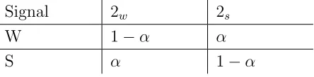
Table 1: Description of the signal
Signal 2w 2s
W 1−α α
S α 1−α
past offers and acceptance behavior of Player 2. Table 1 describes the signal available to Player 1.
The numbers in the table stand for the probability of getting a certain signal given Player 2’s true type. I assume 0 < α < 1/2, thus a smaller α means a more accurate signal. Player 1 does not incur other costs besides the loss of utility from waiting.
With this component added, the representation of histories, strategies and be-liefs have to be adjusted accordingly from the Rubinstein (1985) model. A history
of the game is defined as all the past proposals and responses, plus all the signals Player 1 has drawn. Note that there is no definite relation between the period and the identity of the proposer, except at Period 0. This makes it necessary to spec-ify the identities of the proposer and the responder. Let ht denote the history at
time t before a proposal is made or a signal is drawn, and ˜ht denote the history
at time t after a proposal is made or a signal is drawn. Now if I use φ to de-note the null action, then ht = (x0, s0, A0, x1, s1, A1, ..., xt−1, st−1, At−1), and ˜ht =
(x0, s0, A0, x1, s1, A1, ..., xt−1, st−1, At−1, xt, st), where xt = (xt
1, xt2) ∈ X×φ∪φ×X
is a two-dimensional vector of proposed divisions by both players at period t, st ∈
{W, S, φ} is the signal drawn by Player 1 at period t, and At = (At
1, At2)∈ Y, N is a
two-dimensional vector of actions consisting of rejection by one player and the null action by the other. Note that amongxt
1, st, andAt1, one and only one of them is not
equal to φ. One and only one of xt
2 and At2 is not equal to φ, except when st 6= φ,
in which case both of them are equal to φ. Let Ht and ˜Ht be respectively the set
of all possible histories at period t before and after a proposal is made or a signal is drawn,H be the union of all Ht and ˜Ht, andhbe a generic element ofH. Astrategy
of a player specifies an action for all possible histories after which the player has to move. Denote the action of signal drawing asD. Player 1’s strategy is represented as a sequence of functionsσt
1 :Ht →X∪ {D}ifx2t =φ(or equivalently,t= 0, st−1 6=φ,
or At−1
1 = N), and σt1 : ˜Ht → {Y, N} if xt2 6= φ. Similarly, the strategy of player
2i,(i=w, s) is represented as a sequence of functions σti :Ht→X if A t−1
σt
i : ˜Ht → {Y, N} if xt1 6=φ. In the other cases, the null action is taken. I denote the
entire strategies of Players 1, 2w, and 2s respectively by σ1, σw, and σs. A system of
beliefs of Player 1 in Γ(π) assigns a probability to the event that Player 2 is 2w, after
every possible history. It is represented by a functionµ:H →[0,1], andµ(h0) = π.
A sequential equilibrium of bargaining games requires that µ be Bayesian, and Players 1, 2w, and 2sact optimally given their beliefs and the other player’s strategies.
Furthermore, it requires that theNDOC (Never Dissuaded Once Convinced)property be satisfied, or, onceµ(h) = 1 or 0 for some historyh, it remains so for all subsequent histories.
The equilibrium concept I use is the so-calledbargaining (rationalizing) sequen-tial equilibrium (referred to as “equilibrium” hereafter), which consists a triple of strategies of σ1, σw, and σs, and a system of beliefs of Player 1, µ, such that the
conditions for sequential equilibrium and the assumptions (B-1) through (B-4) below are satisfied.
The assumptions (B-1) through (B-4) below are adopted to significantly reduce the multiplicity of sequential equilibrium in incomplete-information bargaining games. They are the same as those made by Rubinstein (1985) (as by Osborne and Rubinstein (1990)), with one minor exception in (B-2).
The first assumption says that if Player 2 rejects an offer by Player 1 and coun-teroffers in such a way that if Player 1 accepts the offer 2w is worse off than 1’s original
offer, yet 2s is better off, then Player 1 puts probability one on the event that Player
2 is 2s.
Assumption (B-1): If µ(ht−1) 6= 1, (xt,1)
≻s (xt−1,0), and (xt−1,0) ≻w (xt,1),
then µ(˜ht) = 0.
The second assumption says that if Player 2 rejects an offer by Player 1 and coun-teroffers in such a way that both 2w and 2s would be better off if Player 1 accepts
the offer, then Player 1 cannot change his subjective probability that he is playing against 2w.5
Assumption (B-2): If (xt,1)
≻s (xt−1,0) and (xt,1) ≻w (xt−1,0), then µ(˜ht) =
µ(ht−1).
5
This is a strengthened version of the assumption in the original paper. The original assumption
The third assumption is a “tie-breaking” assumption for Player 1.
Assumption (B-3): Player 1 always accepts an offerxif after rejecting he expects to reach an agreement whereby he is indifferent to x.
The fourth assumption limits Player 2’s range of offers, that is, 2w and 2s cannot
use offers that are rejected by Player 1 with certainty to sort themselves.
Assumption (B-4): When it is Player 2’s turn to make an offer,σw(ht)≥Vˆs and
σs(ht)≥Vˆs.
Now, I discuss the equilibrium of the bargaining game without information col-lection. Define the pair (xπ, yπ) as
(xπ,0)
∼w (yπ,1),
(yπ,0) ∼1 π(xπ,1)⊕(1−π)(z(xπ),2),
wherez(x) is defined as thezthat satisfies (x,0)∼w (z,1). Note that from the above,
yπ =z(xπ).
Rubinstein (1985) proves the following result.
Theorem 0. (Rubinstein (1985)) For a game starting with Player 1’s offer: (i) If
π is high enough such that yπ > Vˆ
s, then the only bargaining sequential equilibrium
outcome is h(xπ,0),(yπ,1)
i. (ii) If π is low enough such that yπ <Vˆ
s, then the only
bargaining sequential equilibrium outcome ish(Vs,0),(Vs,0)i.
The theorem states that for a general class of preferences, imposing certain plau-sible assumptions on Player 1’s beliefs, the game never lasts beyond the second period in the equilibrium.6 Rubinstein also notices “it is not clear whether Player 1 would
benefit from having the information about Player 2’s type.” This paper intends to explore what happens if Player 1 has the option to collect information about Player 2’s type. In particular, I would like to study whether and how information collection causes delays.
One important property of the equilibrium outcome is that the pair(xπ, yπ) are
both strictly increasing inπ. This is intuitive since the more likely Player 2 is 2w, the
6
more favorable the situation is for Player 1. By (A-7), Player 1 maximizes expected value ofu(x)δt. The payoff of Player 1 can be represented by the following function
v0(π) =
(
u(Vs), π < π∗;
u(yπ)/δ, π > π∗ .
where π∗
is defined as the boundary point at which yπ = ˆV
s, and hence u(Vs) =
u(yπ)/δ. Thus, v0 is increasing, and strictly increasing if π > π∗
. Note also that
v0(1) = u(Vw). Since the utility functions of the players are concave, which are
necessarily continuous, v0 is also continuous.
In the analysis that follows, I will not distinguish between the prior probability of Player 2 being 2w and Player 1’s belief about Player 2 being 2w, and will simply
call both of them π. Since Player 1’s beliefs will be common knowledge throughout the game, it is valid to treat them equally. Every information set where Player 1’s belief about Player 2 being 2w is the same can be treated essentially the same. I will
denote them by Γ(π).
3
Characterization of Equilibrium
First, I establish a lemma that characterizes Player 1’s information collection behav-ior.
Lemma 1. In the equilibrium, once Player 1 starts the bargaining process, he never halts it to draw additional signals. Formally, if xT
1 6=φ for some T, then st = φ for
all t ≥ T. Furthermore, the equilibrium bargaining outcome must be as described in Theorem 0, with π equal to Player 1’s updated belief about Player 2 being 2w when he
starts the bargaining process.
Proof. Suppose Player 1 starts the bargaining process by offeringx. There could be three types of possible responses from 2w and 2s: i) both reject it; ii) both accept it;
iii) 2s rejects it, and 2w accepts it (the case in which 2s accepts while 2w rejects the
offer is impossible, since 2s is more patient than 2w, and if 2w prefers to wait, then 2s
must also prefer to wait). In case ii), the bargaining game is over. In case iii), Player 1 should be able to infer Player 2’s type, then no additional signals are to be drawn. In case i), Rubinstein (1985) shows in his Proposition 4 that if 2w and 2s both reject
the offer, then they must make the same counteroffer.7 Player 1 should either reject
7
or accept this counteroffer. If he accepts it, then again the bargaining game is over. If he rejects it, then the game is back to the same situation as it was when he started the bargaining process. In particular, Player 1’s subjective probability that Player 2 is 2w should not change. If Player 1 finds it profitable to draw additional signals
now, he should not have started making offers two periods before. This completes the proof of the first part.
Now that Player 1 will not draw more signals once he starts the bargaining, the game is equivalent to the original bargaining game without information collection. So its rationalizing sequential equilibrium must be as specified in Theorem 0.
This lemma states that if Player 1 ever collects information about Player 2’s type, he always does so before he starts to make offers. It lays the foundation for the rest of the paper. Player 1 obtains as many signals as is beneficial to him, and then starts to make offers. Furthermore, once he starts to make offers, the bargaining outcome is described by Theorem 0. In particular, Player 1’s payoff must be consistent with what Theorem 0 requires. Thus, in characterizing the equilibrium of this model, I can focus on the decision problem of Player 1 at the beginning of the bargaining game.
Note that there are only two types of player 2 in this model. Since I focus on pure strategy equilibria, whenever the two types make different offers or accep-tance/rejection decisions, their types are perfectly revealed. If they both accept the offer, then the game is over. If they both reject it, then they will make the same coun-teroffer. If the uninformed player accepts the offer, the game is over. If he rejects the offer, then the game reverses to the state when he initially starts to make offers. He would not have started to make offers if he found it optimal to collect information now. As a result, no additional information collection is needed once the uninformed player starts to make offers.8
Now I define two functions pW and pS, both mapping from [0,1]
×(0,1/2) to [0,1], as follows.
pW(π, α) =π(1−α)/(π(1−α) + (1−π)α)
pS(π, α) =πα/(πα+ (1−π)(1−α))
8
The function pW gives Player 1’s updated belief about the event that Player 2 is 2 w
after seeing the signal “W,” given his initial belief π, andpS is the counterpart when
Player 1 sees the signal “S.” Some properties of these two functions are in order.
Lemma 2. The functions pW and pS satisfy the following properties.
1. pW(π, α)
≥ α, and pS(π, α)
≤ α, with strict inequalities when π 6= 0 or 1. Furthermore, π is a convex combination of pW(π, α) and pS(π, α).9
π = [π(1−α) + (1−π)α]pW(π, α) + [πα+ (1−π)(1−α)]pS(π, α).
2. Both pW and pS are continuous and strictly increasing in π. The function pW
is decreasing in α, and strictly decreasing inα except when π = 1 or 0; and pS
is increasing in α, and strictly increasing in α except when π= 1 or 0.
3. Given α, pW and pS are mutually inverse functions. That is, pW(pS(π)) =
pS(pW(π)) =π.10
4. Givenα, define functions(pW)k(π)and(pS)k(π)where(pW)k(π) =pW
◦pW ◦...◦pW
| {z }
k
(π)
and similarly for (pS)k(π). Then
(a) (pW)k(π) = π(1
−α)k/(π(1
−α)k+ (1
−π)αk),
(pS)k(π) =παk/(παk+ (1
−π)(1−α)k);
(b) (pW)k1(pS)k2(π) =
(pW)k1−k2(π), k1 > k2
π, k1 =k2
(pS)k2−k1(π), k1 < k2
.
Proof. Most of the statements are straightforward from the definition. I only provide the proof of Part 3.
pW(pS(π)) =
πα
πα+(1−π)(1−α)(1−α)
πα
πα+(1−π)(1−α)(1−α) +
(1−π)(1−α)
πα+(1−π)(1−α)α
=π.
Similarly forpS(pW(π)).
9
By convex combination, I mean the linear (nonnegative) coefficients on the terms sum up to 1. The whole expression does not have to be linear. This is used in a number of occasions in the rest of the paper.
10
Here, I suppress the dependence ofpW andpSonα. I will do so in the rest of the paper, where
These properties are very useful in the analysis. For example, Part 3 implies that if it takes one “W” signal to change belief π to π′
, then it takes one “S” signal to change it back. By this property and Property 4, I can construct intervals with bounds {πk
}N
k=0, whereπk = (pS)k(π0) = (pW)N
−k(πN).
Player 1’s decision can be described by the following Bellman’s equation:
v(π) = max{v0(π), δ(π(1−α) + (1−π)α)v(pW(π))+
δ(πα+ (1−π)(1−α))v(pS(π))
} (1)
The first argument in the maximum function is Player 1’s payoff from starting to offer, and the second argument is his payoff from waiting one period and obtaining a signal. Let us define the second argument to be ˜w, a function ofπ,δ and α. For any given value ofπ, if the first argument is bigger than or equal to the second one, then Player 1 starts to offer, and plays according to the rationalizing sequential equilibrium specified in Theorem 0. If, on the contrary, the second term is bigger, then Player 1 draws another signal. Then, according to the signal he gets, he updates his beliefs, and makes the decision again according to the Bellman’s equation, and so on.
Before proceeding to the analysis of the equilibrium, I normalize Player 1’s utility function such that
u(0) = 0, u(1) = 1.
I can do this normalization because players maximize von Neumann-Morgenstern expected utility, which is unique up to monotonic affine transformation. This nor-malization is used in all subsequent analysis. First, I establish a lemma that describes Player 1’s signal drawing behavior in the equilibrium.
Lemma 3. In equilibrium, the following is true about Player 1’s signal drawing de-cisions: there exist πL and πH in (0,1), such that if π < πL or π > πH, then Player
1 does not draw any signals.
Proof. I prove the statement by contradiction.
Suppose there is no πL satisfying the required property. Then there must exist
a strictly decreasing nonzero sequence{πk} that converges to 0, and that satisfies
v(π) = δ(πk(1−α) + (1−πk)α)v(pW(πk)) +δ(πkα+ (1−πk)(1−α))v(pS(πk)).
DefineM =hlogu(Vs)
logδ i
+ 1. Observe that (pw)M is continuous, strictly increasing and
(pw)M(0) = 0 by Parts 2 and 4 of Lemma 2. Thus, I can find K such that for all
k > K , (pw)M(π
k) < π∗. Note π∗ is the threshold value of π in the definition of
above is a convex combination ofδv(pW(π
k)) andδv(pS(πk)). so δv(pW(πk))> u(Vs)
or δv(pS(π
k)) > u(Vs). Since (pW)M(πk) < π∗, pS(πk) < pW(πk) < π∗ by Part 1 of
Lemma 2. Then Player 1 must get this payoff by signal drawing since by Theorem 0 and Lemma 1, Player 1 can get only u(Vs) without signal drawing. Without loss,
supposeδv(PW(π
k))> u(Vs). By the same argument, I have eitherδ2v((pW)2(πk))>
u(Vs) or δ2v(pS(pW(πk))) > u(Vs). Proceed by induction for M steps, and I will
eventually be able to find m, such that |m| ≤ M, and δMv((pW)m(π
k)) > u(Vs),
hence,v((pW)m(π
k))>1 by the definition ofM, which is impossible. So there exists
πL satisfying the desired property.
The argument for the existence of πH is slightly different. The observation is
that Player 1 can never get a payoff higher than u(Vw) by Lemma 1 and Theorem 0.
By the continuity of v0, if π is sufficiently close to 1, thenv0(π) > δu(Vw). Hence it
is impossible that Player 1 draws signals at this π.
The intuition for Lemma 3 is that if Player 1 is quite sure about Player 2’s type, then he does not want to collect information. However, note that it does not show that Player 1’s signal drawing region is an interval in the middle. It does not rule out the possibility that two signal drawing regions surround one region without signal drawing. It is desirable to have that when Player 1 isnot sure about Player 2’s type, he does collect information. In the next section, I identify special cases in which this is true.
Now, I show the existence and uniqueness of the equilibrium.
Theorem 1. There exists a unique function v solving Player 1’s Bellman’s equation (1). Therefore, the bargaining sequential equilibrium outcome of the bargaining game exists, and is unique.
Proof. The proof is an application of the contraction mapping theorem.11 The proof
of Theorem 1 in the case where players have fixed bargaining costs can be found in the appendix.
Consider the space of functions on [0,1] bounded between 0 and 1. Denote it by
V. Define the sup normk k on the space. Denote by T :V →V the function-valued mapping defined by (1), i.e., for w∈V,
T w(π) = max{v0(π), δ(π(1−α) + (1−π)α)w(pW(π))+
δ(πα+ (1−π)(1−α))w(pS(π))}
11
If the mapping T has a unique fixed point in the space V, then the solution to (1) exists and is unique.
Take any two functionsw1, w2 ∈V. Letd=kw1−w2k. Consider kT w1−T w2k. For anyπ ∈[0,1], there are three cases: (i) T w1(π) =T w2(π) =v0(π); (ii)T w1(π)6=
v0(π), T w2(π)=6 v0(π); (iii)T wi(π) = v0(π), T wj(π)=6 v0(π), i6=j.
In case (i),|T w1(π)−T w2(π)|= 0 < δd. In case (ii),
|T w1(π)−T w1(π)|=
δ(π(1−α) + (1−π)α)[w1(pW(π))−w2(pW(π))]
+δ(πα+ (1−π)(1−α))[w1(pS(π))−w2(pS(π))]
By the triangle inequality, I obtain
|T w1(π)−T w2(π)| ≤δ(π(1−α) + (1−π)α)w1(pW(π))−w2(pW(π))
+δ(πα+ (1−π)(1−α))w1(pS(π))−w2(pS(π))
≤δd
The last inequality sign comes from the definition of the sup norm.
In case (iii), without loss of generality assumeT w1(π) = v0(π), T w2(π)6=v0(π), then
δ(π(1−α) + (1−π)α)w1(pW(π)) +δ(πα+ (1
−π)(1−α))w1(pS(π))
≤v0(π)
and
δ(π(1−α) + (1−π)α)w2(pW(π)) +δ(πα+ (1−π)(1−α))w2(pS(π))> v0(π)
Therefore
|T w1(π)−T w2(π)|=|v0(π)−T w2(π)|
≤δ(π(1−α) + (1−π)α)w1(pW(π))−w2(pW(π))
+δ(πα+ (1−π)(1−α))w1(pS(π))−w2(pS(π))
≤δd
I have shown in all three cases|T w1(π)−T w2(π)| ≤δd, sokT w1 −T w2k ≤δd. Since 0< δ <1,T is a contraction. Applying the contraction mapping theorem, I conclude that T must have a unique fixed point in V.
Now that the function v exists and is unique, Player 1’s equilibrium decision rule must be unique. Whether Player 1 draws signals or not at a certain value of π
the equilibrium, starting from the initial prior probabilityπ0, Player 1 keeps drawing signals and doing Bayesian updating, until he obtains a subjective probability πe,
at which no signal is drawn. Then he starts the bargaining process, arriving at an equilibrium outcome according to Theorem 0, withπ =πe.
Theorem 1 shows that for the general preferences discussed above, there exists a unique rationalizing sequential equilibrium of pure strategies. The functionv fully describes the equilibrium, as shown in the proof. Thus, I will frequently usev in place of the equilibrium. An important implication of Theorem 1 is that if the mappingT
is applied to any function belonging to the space V repeatedly, then in the limit the unique solutionv is reached. I can then use the limit argument to prove properties of
v. This kind of reasoning will be used repeatedly in the subsequent analysis. Corol-lary 1 summarizes properties of the functionv.
Corollary 1.1 The functionv is continuous and increasing.
Proof. In the proof, had I defined the spaceV to be allcontinuous functions bounded between 0 and 1, the contraction mapping theorem would still apply. Since limits of uniformly convergent sequences of continuous functions are also continuous functions, (V,k k) is a complete metric space. Hence the solution obtained is the same under these two definitions of V. So v is continuous.
I prove monotonicity from the fact that the solution is unique. For any function
w∈V, the sequence{Tnw
}converges to the solution v. In particular, we can choose
wto be increasing. The first argument of the maximum function,v0, is increasing in
π. For the second argument of the maximum function, ˜w, differentiating with respect toπ,12 I get
˜
w′
(π) = (1−2α)[w(pW(π))
−w(pS(π))]
+[π(1−α) + (1−π)α]w′
(pW(π))(pW)′
(π) +[πα+ (1−π)(1−α)]w′
(pS(π))(pS)′
(π)
.
By Lemma 2, pW(π)
≥ pS(π), and both pW and pS are increasing in π. Since w is
increasing and 0< α <1/2, all three terms in the expression of ˜w′
are nonnegative, which shows ˜w is increasing in π. So T w is increasing. Therefore for all n, Tnw is
increasing inπ. Sincev is the limit of the sequence {Tnw
}, it is also increasing.
The function v is Player 1’s expected equilibrium payoff. The fact that v is continuous comes from the continuity of preferences and the continuity of the
equi-12
librium outcome without information collection. Monotonicity ofv is again intuitive, since Player 1 is in a more favorable position if he faces a weak opponent with higher probability.
4
Special Cases
In this section, I look at some special forms of preferences, and prove properties of the equilibrium under these preferences.
4.1
Fixed Discounting Rate
In this case, players maximize the expectation of discounted value of the share they get of the pie, as opposed to some strictly concave function of the share. Player 1’s preference can be described by maximization of the expectation of the function δtx.
Similarly 2i (i=w, s) maximizes δit(1−x). In this case,
Vs=
1−δs
1−δδs
, Vw =
1−δw
1−δδw
, Vˆs =δVs, Vˆw =δVw;
xπ = (1−δw)(1−δ2(1−π))
1−δ2+δ(δ−δ
w)π
, yπ = δ(1−δw)π
1−δ2+δ(δ−δ
w)π
;
π∗
= (1−δs)(1 +δ)
(1−δs)(1 +δ) + (δs−δw)
;
v0(π) =
(
Vs= 11−−δδδss, π≤π
∗ ,
yπ
δ =
(1−δw)π
1−δ2+δ(δ−δ
w)π π > π
∗ .
In addition, I assumeδ =δw. In this case I obtain a simple form of Player 1’s payoff
function, that is
v0(π) =
(
Vs= 11−−δδδss, π≤π
∗ ,
yπ
δ = π
1+δ π > π
∗
. (2)
whereπ∗
= (1−δs)(1+δ)
(1−δs)(1+δ)+(δs−δ). Note thatπ ∗
is increasing in δ. The function consists of two linear sections that intersect each other atπ∗
. The following lemma proves some general facts about applying the mapping T defined in the proof of Theorem 1 onto functions consisting of two linear sections.
Lemma 4. Define two linear functions w1 and w2 on [0,1],
where 0 < a1 < a2, b2 < b1, and a1+b1 < a2+b2 <1. They intersect each other at
π∗
= b1−b2
a2−a1 (less than 1 since a1+b1 < a2+b2). Now define function w as
w(π) =
(
w1(π) π≤π∗ , w2(π) π > π∗
. (3)
Let v0 in equation 1 be w. The following statements are true:
1. There exists π ∈ [0,1] such that T w(π) > w(π), if and only if the following conditions hold:
α < 1
2 −
(1−δ)(b1a2−a1b2)
2δ[(a2+b2)−(a1+b1)](b1−b2), (4)
δ[(a2+b2)−(a1+b1)](b1−b2)>(1−δ)(b1a2−a1b2). (5)
2. The difference between T w and w, T w−w, is increasing on [pS(π∗), π∗], and
decreasing on [π∗, pW(π∗)], and attains its maximum at π∗.
3. The region in whichT w−w >0is an open interval(π1
1, π12)lying in[pS(π∗), pW(π∗)].
Proof. In this case, function ˜wcan be written as
˜
w(π) =δ[π(1−α) + (1−π)α]w(pW(π)) +δ[πα+ (1−π)(1−α)]w(pS(π))
=
δ(a1π+b1), π ≤pS(π∗),
δ{[αa1+ (1−α)a2−(1−2α)(b1 −b2)]π+ [(1−α)b1+αb2]},
pS(π∗)
≤π ≤pW(π∗),
δ(a2π+b2), π ≥pW(π∗).
It has three linear sections intersecting their neighbors atπ =pS(π∗) andπ=pW(π∗),
and d= max{0,w˜−w}.
Let us first prove Parts 2 and 3. First suppose that there exists π = π0, such
that T w(π) > w(π). Observe that ˜w−w is negative forπ ≤pS(π∗) orπ
≥pW(π∗),
since δ < 1 and w is piecewise linear. So d = 0 for these cases. Therefore π0 must
lie in [pS(π∗), π∗] or [π∗, pW(π∗)]. Now I argue that ˜w
−w must be increasing on
[pS(π∗), π∗] and decreasing on [π∗, pW(π∗)]. Since ˜w
−wis linear on both intervals, it must be monotonic (including the case that it is constant) on these two intervals. I prove the claim by showing that the other cases are impossible. If ˜w−wis decreasing on [pS(π∗), π∗], then it is always negative on this interval. In particular, it is negative
atπ∗. But since ˜w
−w is monotonic on [π∗, pW(π∗)], and negative at π =pW(π∗), it
is always negative on [π∗, pW(π∗)]. This contradicts the existence of π
increasing on [pS(π∗
), π∗
]. Similarly, it is decreasing on [π∗
, pW(π∗
)]. Thus it attains
its maximum at π∗
. Furthermore, there must exist π1
1 ∈ (pS(π ∗
), π∗
) and π1 2 ∈
(π∗
, pW(π∗
)) at which ˜w−w is zero. The expressions for the two values are
π11 = (1−δ)b1+δα(b1−b2)
δ(1−α)(a2−a1)−δ(1−2α)(b1−b2)−(1−δ)a1,
π12 = δ(1−α)(b1−b2)−(1−δ)b2
(1−δ)a2+δα(a2−a1) +δ(1−2α)(b1−b2).
In the open interval between these two values ˜w−wis positive. Outside this interval, ˜
w−wis negative. Sinced= max{0,w˜−w}, the functiondmust also be increasing on [pS(π∗
), π∗
], decreasing on [π∗
, pW(π∗
)], and attains its maximum atπ∗
. Furthermore, it is positive only on the open interval (π1
1, π21). This completes the proof of (ii) and
(iii).
Now I prove Part 1. First I show the conditions are necessary. From the above proof, I know that if there existsπ ∈[0,1], such thatT w(π)> w(π), thend=T w−w
is maximized atπ∗
. ThenT w(π∗
)−w(π∗
)>0 must hold, which implies
δ(1−2α)[(a2+b2)−(a1+b1)](b1−b2)−(1−δ)(b1a2−a1b2)>0.
Thus
α < 1
2−
(1−δ)(b1a2−a1b2) 2δ[(a2+b2)−(a1+b1)](b1−b2)
,
but the right hand side of the above inequality to be positive, which implies that the following inequality must hold
δ[(a2+b2)−(a1+b1)](b1 −b2)>(1−δ)(b1a2−a1b2).
The above two inequalities are also sufficient for the existence ofπ0 ∈[0,1] such that T w(π0)> w(π0). Just chooseπ0 =π∗.
Lemma 4 says that if the mappingT is applied on a function w with two linear sections with ascending slopes, with the function itself serving asv0, then the region in which T w > w must lie in the middle. Furthermore, the “gain” T w−w is max-imized at the intersection of the two linear sections. This fact is important in the characterization of the equilibrium for the class of preferences I consider in this part. Note that although in most cases, the coefficientsa1, b1, a2, b2 should depend onδ, δw,
and δs, the proof is not affected by such dependence. This is useful in the proof of
Theorem 2. If players’ preferences are such that without information collection, Player 1’s payoff v0 takes the form of w in (3),13 then the following are true about
Player 1’s signal drawing decisions:
1. Player 1’s signal drawing region is nonempty if and only if (4) and (5) hold;
2. Player 1’s signal drawing region is in the form of (πL, πH), where 0 < πL <
πH <1, if his signal drawing region is nonempty.
Proof. Since v0 =w, by Theorem 1, if T w = w then the solution to equation (1) is
v =w, and Player 1 does not draw signals. The converse is also true. By Lemma 4, this implies that Player 1 draws signals if and only if (4) and (5) hold.
If Player 1 does draw signals, then as shown in the proof of Lemma 4,T wconsists of three linear sections. The middle one is equal to ˜w, with slope and intercept being
ha12, b12i=hδαa1 +δ(1−2α)(b1−b2), δ(1−α)b1+δαb2i.
The inequality T w > w holds only on the open interval (π11, π21). From the proof of
Lemma 4, if I let a11 = a1, b11 = b1, a13 = a2, and b13 = b2, then I claim that {a1j}3j=1
and{a1j+b1j}j3=1 are increasing sequences, and {b1j}3j=1 is a decreasing sequence. The
sequence{a1j}3j=1 is increasing because of the monotonicity property of ˜w−w. Since
for j = 1,2, a1jπ+b1j intersects with a1j+1π+b1j+1 on (0,1) by Lemma 4, it must be
that b1j > b1j+1, and a1jπ+b1j < a1j+1π+b1j+1 for all π to the right of the intersection
point. In particular,a1j +b1j < a1j+1+b1j+1 holds.
Now I prove by induction the claim “for allk,Tkw > w is only true on an open
interval(πk
1, πmkk−1), where 0< π
k
1 < πkmk−1 <1.” Suppose Tkw consists of m
k linear sections intersecting with neighboring
sec-tions, and let these sections be represented by slope and intercept pairs (ak j, bkj),
j = 1,2, ..., mk. Suppose that {akj} mk
j=1, {akj +bkj} mk
j=1 are increasing sequences and
{bk j}
mk
j=1 is a decreasing sequence. Let the boundary points between these sections be πk
j, j = 1,2, ..., mk−1. The sequences and boundary points are ordered from left to
right. Finally,Tkw=wforπ
≤πk
1 and π≥πmkk−1. On the open interval (π
k
1, πkmk−1),
T w > w is true.
Now look at Tk+1w. Applying to the linear sections ofTkw the same reasoning
used in the proof of Lemma 4, the result in Lemma 4 is true for any two linear sections. Thus, after the k + 1-th iteration, Tk+1w also consists of linear sections
intersecting with neighboring sections, and the sequences {akj+1} mk+1 j=1 , {b
k+1
j } mk+1 j=1 ,
13
and{akj+1+b k+1
j } mk+1
j=1 preserve the properties of the sequences of Tkw. Furthermore,
if I denote by πk
i,j the intersection between akiπ+bki and akjπ+bkj, then π k+1
mk+1−1 <
pW(max
jπj,mk k) = p
W(πk
mk−1,mk) < 1, and π
k+1
1 > pS(minjπjk1) = pW(π21k ) > 0. Tk+1w > w is true only on (πk+1
1 , π
k+1
mk+1−1). The claim is proved.
The final step is to state that it takes finite steps to get to v for any initial w. This is true due to the reasoning used in the proof of Lemma 3. There existsM great enough, such that δM < w(π) for all π.
Now I have shown thatv > w only on an open interval (πL, πH). Hence, Player
1 only draws signals on this interval.
The above theorem applies to not only the fixed discounting rate preferences with the assumption δ = δw, but also any preference settings in which Player 1’s
payoff according to Theorem 0 as a function of π consists of two linear sections intersecting each other. In all these cases, Player 1’s signal drawing behavior can be fully characterized by two threshold values of π. In the interval between these two values, Player 1 draws signals; outside this interval, he does not. This result means that starting from any belief, Player 1 trades off between earlier agreement and more favorable agreement with more information. Player 1, the uninformed player, collects information until he is sufficiently sure about Player 2’s type. His main objective is to take advantage of the weak type as much as possible.
Condition (4) suggests that Player 1 draws signals if and only if the information is accurate enough, other parameters being equal. Condition (5) is hard to interpret asa1, b1, a2, and b2 usually depend on δ, δw, and δs (but not α).
For the fixed discounting rate case with the assumption δ = δw, conditions (4)
and (5) take the following form:
α < (2δ−1)(δs−δ)−(1−δs)(1−δ 2)
2δ(δs−δ)
, (6)
0 < (2δ−1)(δs−δ)−(1−δs)(1−δ2). (7)
But these in turn require the following two conditions:
δs >
√
3/2, (8)
δ ∈ 2δs+ 1−
p
4δ2
s−3
2(1 +δs)
,2δs+ 1 +
p
4δ2
s −3
2(1 +δs)
!
. (9)
This means thatδsmust be great enough andδmust be in a suitable range. That
is, it can be neither too close nor too far from δs. If δ is too close to δs, then there
if δ is too far from δs, Player 1 loses too much from waiting, and probably loses too
much from knowing that Player 2 is strong. Conditions (6), (8) and (9) are necessary and sufficient conditions for there to be information collection in the equilibrium.
Corollary 2.1. Given the same condition as that in Theorem 2, the function v is decreasing in α at every π ∈ [0,1], and the lower (upper) threshold of the signal drawing region is increasing (decreasing) in α.
Proof. Step 1 First I prove T w is decreasing in α at every π ∈[0,1]. Observe that the middle linear section generated byT has the following expression:
˜
w(π, α) = [δαa1+δ(1−α)a2 −δ(1−2α)(b1−b2)]π+δ(1−α)b1+δαb2
Differentiating with respect toα gives
∂w˜
∂α =−δ[(a2+b2)−(a1+b1)]π−δ(b1−b2)(1−π)<0,
because of the conditions a1+b1 < a2 +b2 and b2 < b1. SinceT w = max{v0,w˜}, for every π ∈[0,1], T w is decreasing in α no matter v0 ≥ w or v0 < w at π. Note that this result doesnot depend on the fact v0 =w.
Step 2 Let Tα1 and Tα2 denote respectively the mapping T when α = α1 and
α=α2, andα1 ≤α2. Letvα1 and vα2 denote respectively the corresponding solution.
By Step 1, I haveTα1w≥Tα2w, hence
(Tα1)
2w
≥Tα1Tα2w.
Following similar argument to that in Step 1, I can prove
Tα1Tα2w≥(Tα2)
2w.
Since they are generated respectively by applyingTα1 and Tα2 onTα2w, I can use the
result of Step 1. For any two linear sections ofTα2w,Tα1 gives a higher middle section
thanTα2 does. It is possible that at some pointπ,p
W(π, α1) is so large orpS(π, α2) so
small (by part 2 of Lemma 2,pW(π, α1)> pW(π, α2) andpS(π, α1)< pS(π, α2) for all
π∈ (0,1)) that pW(π, α1) is on a different linear section from pW(π, α2) or pS(π, α2)
is on a different linear section frompS(π, α1). But whenever this happens, pW(π, α1)
will be on a higher section than if the section that pW(π, α2) is on is extended to
pS(π, α1). Similarly for pS(π, α1). For the same linear sections, T
α1 gives a higher
middle section than Tα2 does. Now that p
W(π, α1) or pS(π, α1) is on a higher linear
section, then Tα1 is even higher than Tα2, hence Tα1Tα2w ≥ (Tα2)
2w. Now I have
shown that
(Tα1)
2w
≥(Tα2)
Proceeding by induction, I can show that (Tα1) kw
≥ (Tα2)
kw for all k if α1
≤ α2. Since the limits of the iteration (in fact, it is over in finite steps) are the solutionsvα1
and vα2, vα1 ≥vα2 if α1 ≤α2. That is, v is decreasing in α at every π∈[0,1].
Recall in Part 2 of Theorem 2, the signal drawing region is an open interval in the middle. Sincev is decreasing in αat everyπ ∈[0,1], the lower (upper) threshold of the signal drawing region is increasing (decreasing) inα.
What the above corollary says is that for the class of preferences that result in
v0 of the form of w in equation (3), the equilibrium has nice properties in terms of comparative statics. Thatv is decreasing in αat every π shows that the uninformed player is always better off having a more accurate signal about the informed player. Also, since the signal drawing region is also bigger under a smallerα, the uninformed player is more willing to collect information at any initial belief, if the information source is more accurate. The second property is in fact an implication of the first one. Since the uninformed player draws signals if and only if v > v0, and v is always greater for a more accurate signal, Player 1 is more likely to draw signals with a more accurate signal.
4.2
Fixed Bargaining Costs
In this subsection, I look at preferences that can be represented by the utility function
x−ctfor the divisionx at periodt. In this case, Player 2w has higher cost (cH) than
Player 1’s (c), and 2s has lower cost (cL). So for this discussion, I will call them
2H and 2L, the prior probability for Player 2 to be 2H is π. The costs also satisfy
c1+cH +cL<1. The proofs for Lemmas 1 and 3 are slightly different from the ones
presented above, while the proof of Theorem 1 is quite different, in that the application of the contraction mapping theorem is not as handy. I put the proof of Theorem 1 for this case in the appendix. For this case, in the bargaining sequential equilibrium outcome without information collection, Player 1’s payoff function becomes
v0(π) =
(cH +c1)π+ (1−cH −c1), π ≥π0;
(cH +c1)π−c1, π∗ ≤π < π0;
cL, π < π∗.
where
π0 = 2c1/(cH +c1),
and
π∗
The special feature of v0 in this case is that it has two threshold values, and a discontinuity at one of them, π0. This jump is a major motivation for information collection. In the appendix, I include the proof of Theorem 1 for this case. Corollar-ies 1.2 and 1.3 further describe Player 1’s equilibrium information collection behavior.
Corollary 1.2 In the case of fixed bargaining costs described above, the function v
is increasing, strictly bigger than v0 in an interval (ω, π0) if there are values of π at which v > v0, and equal to v0 in (0, ω)∪[π0,1]. In other words, Player 1’s signal drawing decision can be characterized by two thresholds ω and π0, if he draws signals at all.
Proof. The proof is constructive. By Theorem 1 and in particular, condition (C), if I start with anyw∈V, by iteration of T, I am able to get the functionv. Let us start with the function w1 defined by
w1(π) = (cH +c1)π+ (1−cH −c1)
for allπ ∈[0,1]. This is an upper bound of the payoff Player 1 can get. The corollary can be proved by using the following facts.
1. For all k, Tkw1 is increasing in π.
2. {Tkw1
}is a decreasing sequence. So if there existsω, such thatTkw1(π) = v0(π)
for all π≤ω, then this remains true for Tk+1w1.
3. For any ω < π0, if Tkw1(ω) =v0(ω), then Tkw1(π) = v0(π) for all π≤ω.
This corollary shows that for the case of fixed bargaining costs, Player 1’s signal drawing region also lies in the middle. That is, Player 1 collects information until he is quite sure about Player 2’s type.
Corollary 1.3 If max{3cH/2 + c1/2,2c1 +cH} < 1, then there always exists a
ω0 ∈ [π1, π0), such that v(π) > v0(π) for all π ∈ (ω0, π0), regardless of the value of
α. In other words, if this condition is satisfied, there is always a nontrivial region in which Player 1 draws signals.
Proof. Similar to the Proof of Corollary 1.2. This time let us choosew2 = v0 as the
1. {Tkw2
}is an increasing sequence.
2. Given the required condition, in the first round of iteration, T w2(π0−) > v0(π0−), regardless of the value of α.
Corollary 1.3 shows that there is a particular property about the fixed bargaining costs preference. If the cost of waiting is not too large, then there always exist initial beliefs at which there is gain from information collection, regardless of the accuracy of the information source. This result comes from the discontinuity of Player 1’s payoff in the probability of Player 2 being 2H without information collection. As we have
seen, at one threshold value of π, Player 1’s payoff jumps from almost nothing to almost everything.
It would be interesting to explore how Player 1’s information collection behavior changes as α changes, and how Player 1’s payoff depends on α. But these problems remain unresolved, due to the lack of an analytical solution.
5
Discussions and Further Research
This paper looks at one particular reason why agreement may be delayed in bargain-ing: the possibility to collect more information. I identify cases in which delays do happen, and perform comparative statistic analysis on two special cases, namely the fixed-bargaining-cost and fixed-discounting-rate cases.
Note that the setup of this paper is different from that of the models in which the uncertainty is about the valuations of the two parties. In particular, without information collection, there is at most one period of delay in the selected “bargaining sequential equilibrium.” With information collection, there is a possibility (albeit small) that the bargaining process drags on for a long period of time.
same about information collection. Therefore, if the “Coase conjecture” critique is valid, the delay caused by information collection will vanish as the players are allowed to make frequent offers.
Appendix: Proof of Theorem 1 for the case of Fixed Bargaining Costs
Theorem 1 There exists a unique function v solving Player 1’s Bellman’s equa-tion (1).
Proof. The proof is an application of the contraction mapping theorem. First, observe that by definition,
i)v(π)≥v0(π) everywhere in the interval [0,1].
By Theorem 0 and Lemma 1 (also see the proof of Lemma 3),
ii)v(π)≤(cH +c1)π+ (1−cH −c1) everywhere in the interval [0,1].
By Lemma 3,
iii) v(π) =v0(π) if π∈[π0,1].
Let the space V be the set of functions satisfying Properties i), ii) and iii). I denote by T :V →V the function-valued mapping defined by (1), i.e.,
T w(π) = max{v0(π), (π(1−α) + (1−π)α)w(pH(π))+
(πα+ (1−π)(1−α))w(pL(π))−c
1}
A solution to (1) is equivalent to a fixed point of Tin the space V. Define the sup normkk on the space V, then V is a complete metric space. Also, define
πk = (pL)k(π0), k = 1,2, ..., n.
Part 1
With the following procedure, I will find ˜π > 0 and finite K ∈ N, such that
Tkw(π) = u(π) for all k
≥Kand π <π˜. I use an inductive argument.
Step 1.1 Given Property ii) and Part 1 of Lemma 2, I can immediately show that any function w∈V must satisfy the following
(π(1−α) + (1−π)α)w(pH(π)) + (πα+ (1−π)(1−α)w(pL(π))−c
1
≤(cH +c1)π+ (1−cH −c1)−c1
for every π∈[0, π0). So
T w(π)≤max{v0(π), (cH +c1)π+ (1−cH −c1)−c1}
for every w∈V and π∈[0, π0). Note that the form of v0 is
v0(π) =
(cH +c1)π+ (1−cH −c1), π≥2c1/(cH +c1);
Now forπ ∈[0, π0), if
(cH +c1)π+ (1−cH −c1)−c1 ≥v0(π),
then
T w(π)≤(cH +c1)π+ (1−cH −c1)−c1. (T-1)
But that only requires
1−cH −c1 ≥0
forπ ∈[(cL+c1)/(cH +c1), π0) and
(cH +c1)·0 + (1−cH −c1)−c1 ≥cL
forπ ∈[0,(cL+c1)/(cH+c1)). The first condition holds by assumption. If the second
condition fails to hold, there must exist π′
, such that for all π < π′
, T w(π) = u(π) =
cL. The same is true for all k > 1, Tkw(π) as well (I omit the calculation). I stop
here, and let ˜π =π′
and K = 1. If the second condition does hold, then we proceed to Step 1.2.
Step 1.2 Now applying Part 1 of Lemma 2 again, and using (T-1), I obtain
(π(1−α) + (1−π)α)T w(pH(π)) + (πα+ (1−π)(1−α)T w(pL(π))−c
1
≤(cH +c1)π+ (1−cH −c1)−c1−c1
for every π∈[0, π1), i.e., pH(π)∈[0, π0). So
T2w(π)≤max{u(π),(cH +c1)π+ (1−cH −c1)−2c1}
Following the same logic in Step 1, we have if
(cH +c1)π+ (1−cH −c1)−2c1 ≥v0(π),
then for all π∈[0, π1),
T2w(π)≤(c
H +c1)π+ (1−cH −c1)−2c1. (T-2)
Similarly to Step 1.1, this requires that
1−cH −2c1 ≥0,
forπ ∈[(cL+c1)/(cH +c1), π1) if (cL+c1)/(cH +c1)< π1 , and
(cH +c1)·0 + (1−cH −c1)−2c1 ≥cL
for π ∈ [0,(cL+c1)/(cH +c1)). Note that the first condition is redundant if the
the second condition fails, I am able to findπ′
such that T2w(π) =u(π) =c
L for all
π < π′
. Set ˜π =π′
and K = 2. If it does hold, then I proceed to Step 1.3, and so on.
Step 1.K From the above procedure I know that K = [(1−cH −cL)/c1], and ˜π
can be chosen accordingly.
Now I have shown for all w ∈ V and k > K, Tkw(π) = c
L holds for all π < π˜.
This implies without loss, I can focus on functions that satisfy
w(π) =cL for all π <π˜ (∗)
in the subsequent analysis.
Part 2
Define M = minm∈N{(pH)m(˜π) ≥ π0}. I know M < ∞ because (pH)m(π)
converges to 1 as m → ∞ for any π > 0 by Part 4 of Lemma 2. Now consider the mappingTM. I shall show that it is a contraction. Take any two functionsw
1, w2 ∈V
satisfying (*). Letd=kw1−w2k. Observe thatw1 =w2 everywhere on [0,π˜)∪(π0,1]
Let us take any π∈[˜π, π0). There are three cases:
Case 1. If TMw
1(π) = TMw2(π) = v0(π), then any 0 < ρ < 1 will make
TMw1(π)−TMw2(π) < ρ·d. Also note it satisfies the (C-M) condition as defined
in Case 2.
Case 2. IfTMw
1(π) = v0(π), but TMw2(π)6=v0(π), then
u(π)≥(π(1−α) + (1−π)α)TM−1w1(pH(π))+
(πα+ (1−π)(1−α))TM−1w1(pL(π))
−c1
and
u(π)<(π(1−α) + (1−π)α)TM−1w2(pH(π))+
(πα+ (1−π)(1−α))TM−1w2(pL(π))−c1
Then
TMw1(π)−TMw2(π)
<
(π(1−α) + (1−π)α)[TM−1w1(pH(π))−TM−1w2(pH(π))]+
(πα+ (1−π)(1−α))[TM−1w1(pL(π))−TM−1w2(pL(π))]
.
By the triangle inequality, I obtain
TMw1(π)−TMw2(π)
≤(π(1−α) + (1−π)α)TM−1w1(pH(π))−TM−1w2(pH(π))+
(πα+ (1−π)(1−α))TM−1w1(pL(π))−TM−1w2(pL(π))
(C-M)
Similarly, the case that TMw1(π) 6= v0(π), but TMw2(π) = v0(π) also satisfies
Case 3. IfTMw1(π
H)6=v0(πH) and TMw2(πH)6=v0(πH), then by direct
substi-tution (C-M) is satisfied.
Before proceeding, note that the RHS of (C-M) is a convex combination of
TM−1w1((pH)1(π))−TM−1w2((pH)1(π))
and
TM−1w1((pL)1(π))−TM−1w2((pL)1(π)).
Repeat the above analysis for
TM−1w1(pH(π))−TM−1w2(pH(π))
and
TM−1w1(pL(π))−TM−1w2(pL(π),
I obtain two (C-(M-1)) conditions for all three possible cases listed above. Substitute them back into (C-M), I obtain that TMw1(π)−TMw2(π) is less than or equal to
a convex combination of TM−2w1((pH)m(π))−TM−2w2((pH)m(π)), |m| ≤ 2, with
the interpretation (pH)m = (pL)−m if m < 0 and the identity function if m = 0. In
particular, the coefficient onTM−2w1((pH)2(π))−TM−2w2((pH)2(π)) isπ(1−α)2+
(1−π)α2 and that onTM−2w1((pH)−2(π))−TM−2w2((pH)−2(π))isπα2+(1−π)(1− α)2.
I proceed by induction forM steps, until I obtain 2M(C-1) conditions, substitute them into the condition gotten from the previous step and obtain that|TMw1(π)
−TMw2(π)
|
is less than or equal to a convex combination of expressions in the form of
w1((pH)m(π))−w2((pH)m(π)), where|m| ≤M. The coefficient on
w1((pH)M(π))−w2((pH)M(π)) is π(1− α)M + (1 −π)αM and the coefficient on
w1((pH)−M(π))−w2((pH)−M(π)) is παM + (1 − π)(1 − α)M. By the definition
of M, (pH)M(π)
≥ π0 and (pH)−M(π)
≤ π˜ must be true for all π ∈ [˜π, π0). So
w1((pH)M(π))−w2((pH)M(π)) = w1((pH)−M(π))−w2((pH)−M(π)) = 0 by (*)
and Property iii). Further, by the fact
w1((pH)m(π))−w2((pH)m(π))≤ kw1−w2k=dfor all |m| ≤M,
I conclude for allπ ∈[˜π, π0),
TMw1(π)−TMw2(π)
≤[1−(π(1−α)M + (1−π)αM)−(παM + (1−π)(1−α)M)]·d
= [1−αM −(1−α)M]·d
.