A framework for interpolating scattered data using space filling curves

BIROn - Birkbeck Institutional Research Online

Weston, David (2016) A framework for interpolating scattered data using

space-filling curves. In: Boström, H. and Knobbe, A. and Soares, C. and

Papapetrou, P. (eds.)

Advances in Intelligent Data Analysis XV. Lecture

Notes in Computer Science 9897. New York, U.S.: Springer International

Publishing, pp. 249-260. ISBN 9783319463483.

Downloaded from:

Usage Guidelines:

A Framework for Interpolating Scattered Data

using Space-filling Curves

David J. Weston

Department of Computer Science and Information Systems, Birkbeck College, University of London, London, United Kingdom.

Abstract. The analysis of spatial data occurs in many disciplines and covers a wide variety activities. Available techniques for such analysis include spatial interpolation which is useful for tasks such as visualiza-tion and imputavisualiza-tion. This paper proposes a novel approach to interpo-lation using space-filling curves. Two simple interpointerpo-lation methods are described and their ability to interpolate is compared to several interpola-tion techniques including natural neighbour interpolainterpola-tion. The proposed approach requires a Monte-Carlo step that requires a large number of iterations. However experiments demonstrate that the number of itera-tions will not change appreciably with larger datasets.

1

Introduction

Spatial interpolation is one of the many tools available for spatial data mining [10]. It is particularly useful in spatial analysis since it is often the case that data cannot be collected at every desired location due to practical issues such as cost. In addition the data may have missing values [11], that may require imputation. The literature for spatial interpolation is large and the interested reader is referred to [8] for an overview of available approaches in the practical context of environmental sciences.

Space-filling curves have been successfully used in a broad range of compu-tational problems, for example in calculating efficiently all nearest neighbours [4] and image segmentation [9], see [1] for a comprehensive review. The primary reason for this is the fact that space-filling curves can be used to map multi-dimensional Euclidean data onto one dimension which partially preserves local spatial correlations, i.e. points that are close in the multidimensional space are likely to be close in the one dimensional ordering of the data.

a simple interpolation scheme is used to impute the value at each query point. This process is repeated using different shape preserving transformations and the resulting interpolations are then aggregated. The main motivation for this work is to produce a conceptually simple approach for interpolation in two or higher dimension that is also numerically robust and simple to implement.

In the next section, relevant methods for interpolating scattered data are dis-cussed. After which space-filling curves are introduced with a brief overview of the construction of the Hilbert curve. Following this, the framework for perform-ing spatial interpolation usperform-ing space-fillperform-ing curves is introduced. Experiments to demonstrate the utility of the approach are provided. The final section concludes with ideas for future research.

2

Scattered data interpolation methods

In the following discussion it will be assumed that there arendata-sitesx1, . . . , xn with respective locationsx1. . .xnand each data-site has a value denotedz1. . . zn. In addition there aremquery sites,q1. . . qmwith locationq1. . .qm. It is at these locations that an imputed value is desired, i.e. we wish to estimate ˆf(q_j), for query siteqj.

There are a large array of methods available for spatial interpolation. The focus in this section will be on three methods for spatial interpolation. They have been chosen specifically because they are the higher dimensional analogues of the interpolation we do in one dimension and hence provide a clear comparison. They arepiecewise constant, piecewise linearandnatural neighbourinterpolation.

Piecewise constantinterpolation is a very simple approach to scattered data interpolation. The interpolated value, ˆf(qj), for query site qj is the value asso-ciated with the closest (in the Euclidean sense) data-site.

Piecewise linearinterpolation for scattered data uses the Delauney triangula-tion, see e.g. [12], induced from the data-sites. The vertices in this triangulation are the data-sites. In, for example 2D, a query point will reside in one triangle. Let us assume that the vertices are the data-sites with indiciesp1j, p2j, p3j, then

ˆ

f(q_j) = ∑3

i=1apizpij

∑3

i=1api

,

where api is the Euclidean distance between the query pointqj and the vertex

locationxpij

The location of the query point is added to the list of data-sites and a new Voronoi diagram is produced. This is shown in Fig. 1(b) where the query point in this figure is denoted with a cross. This query point has its own Voronoi tile that contains regions taken from the original Voronoi tiles shown in Fig. 1(a). Data-sites that have had their Voronoi tile changed by the inclusion of the query point are called its natural neighbours. For a particular query pointqj

ˆ

f(q_j) = ∑

iwijzi

∑

iwij

,

where wij is the area from the query point tile that was originally part of the Voronoi tile for theith data-site.

Conceptually natural neighbour interpolation is relatively straightforward however computing it efficiently is rather involved [7]. Indeed approximations that rely on discretising the region of interest have been proposed to produce more efficient algorithm [13]. Natural neighbour interpolation is defined for two or more dimensions, since in 1D, the procedure for natural neighbour interpola-tion reduces to piecewise linear interpolainterpola-tion. Briefly, in 1D the Voronoi tiles are simply intervals and the natural neighbours of a query point are its predecessor and successor data-sites. Since we shall be using linear interpolation in 1D in our proposed approach, we consider natural neighbour interpolation to be a relevant method to compare against.

(a) Data-sites only (b) Data-sites and query point

Fig. 1: Voronoi diagrams used for natural neighbour interpolation weight calcu-lation. The query pointqj is denoted by a cross located in the centre of (b).

3

Space-filling curves

(a) (b) (c)

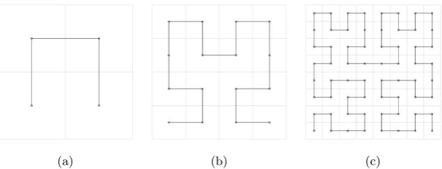
Fig. 2: First three iterations for Hilbert curve construction, the circles denote the centres of the sub-squares.

Fig. 2 shows the construction of the Hilbert space-filling curve. A square is sub-divided into four sub-squares which are given a specific order and orientation. Joining the centres of these sub-squares by following their order produces a polygon approximation to the Hilbert curve, Fig. 2(a). These sub-squares are themselves recursively subdivided. Figs 2(b,c) show the polygon curve for second and third iteration respectively. In the limit as the number of iterations tends to infinity, the polygon curve tends to the Hilbert curve.

A detailed explanation regarding space-filling curves and their construction can be found in [1], [14]. The code used in the paper is based on [15].

4

Framework for Interpolation

There are three stages in the proposed framework for interpolation, denoted shape preserving embedding,one-dimensional interpolationandaggregation. Each stage is described separately in the following sections.

4.1 Shape Preserving Embedding

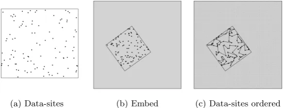
The first stage involves ordering the data-sites (and query locations) in multidi-mensional space along a space-filling curve. The entire process is demonstrated graphically for the 2D case in Fig. 3. For simplicity it is assumed that interpo-lation is required over a square region of interest containing all the data-sites, Fig. 3(a). A shape preserving transformation is applied that maps the region of interest onto the unit square denoted by the grey region in Fig. 3(b). Each data-site (and query point) can then be ordered along a Hilbert curve. Fig. 3(c) shows each data-site joined to their predecessor and successor along the space-filling curve.

(a) Data-sites (b) Embed (c) Data-sites ordered

Fig. 3: Embedding data-sites onto Hilbert Curve.

composite, comprising a translation, a rotation, a reflection (with probability 0.5) and a scaling. Details of the embedding can found in [16], the maximum scale factor in this study is 10. For reasons of computational simplicity the region of interest, i.e. domain over which the interpolation function ˆf(·) is to be estimated is assumed to be a discretised square with resolution 2000×2000.

Lethdenote a function that maps a point in the unit square onto the unit interval using a Hilbert curve. The Hilbert index,ti, for theith data-site is

ti=h(e(xi))

and similarly for query sites. The data is then sorted in ascending Hilbert index order. Let this ordering function be denoted byπ, thentπ(di)andtπ(qj)are both

non-decreasing fori= 1,· · ·, nandj= 1,· · ·, mrespectively.

4.2 One-Dimensional Interpolation

Once a Hilbert index has been associated with each datum, interpolation can proceed using any 1D interpolation method. For this study 1D piecewise constant and 1D piecewise linear interpolation (described in Section 2), denoted Hilbert-ConstandHilbert-Linearrespectively are used. Both these methods are trivially simple to implement and due to their simplicity they are amenable to further analysis which can be achieved without the need of a ground truth function to interpolate, see Section 6.

4.3 Aggregation

Letg denote a function that encapsulates the two stages described above, such that interpolated value for the query siteqj is

ˆ

f(q_j) =g(q_j,x1...m, z1...m, h, Q1, e).

WhereQ1denotes a plug-in one-dimensional interpolation function andea shape

(a) Ground Truth (b) Constant (c) Linear (d) Natural Neigh-bour

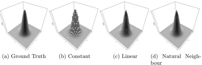
Fig. 4: Bivariate Gaussian test function and interpolated functions using stan-dard 2D approaches based on data-sites located on a regular 21×21 grid.

and data-site values respectively; his the Hilbert mapping, note that this can be replaced with other space-filling curve mappings.

Lete1, . . . , eη be identically and independently drawn legitimate transforma-tions, further details for the sampling regime can be found in [16]. The aggregated interpolated value for the query siteqj is simply the average interpolated value, i.e.

ˆ

f(q_j) = 1

η

η

∑

k=1

g(q_j,x1...m, z1...m, h, Q1, ek).

5

Experiments

The following experimental design has been motivated by [6]. The interpolation schemes are tested by evaluating the mean squared error (MSE) and the maxi-mum absolute error (Max Error) between interpolated values and a ground truth function. For the ground truth Franke’s function [6] has been selected, see Fig. 6(a).

It is also instructive to visualise the interpolation, for this task a bivariate Gaussian is used see Fig. 4(a). The experiments are organised as follows. First the focus is on visualising the resulting interpolations, then a more formal approach to evaluating the interpolation methods is performed. Henceforth piecewise linear and piecewise constant shall be referred to as linear and constant respectively.

5.1 Visualising the Interpolated Function

(a) 1 iteration (b) 100 iterations (c) 1000 iterations (d) 10,000 iterations

(e) 1 iteration (f) 100 iterations (g) 1000 iterations (h) 10,000 iterations

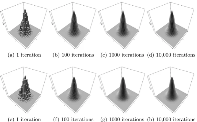
Fig. 5: Hilbert-Const Interpolation of a Bivariate Gaussian based on data-sites located on a regular 21×21 grid. Top row Hilbert-Const Interpolation, bottom row Hilbert-Linear Interpolation.

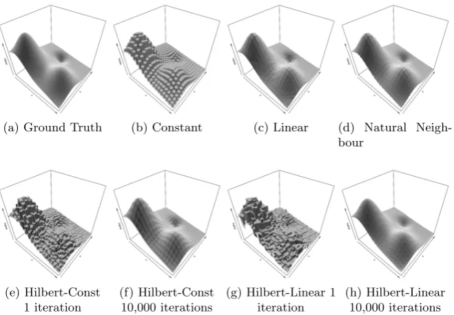
It is clear that constant interpolation, Fig. 4(b), does a poor job of recon-structing the ground truth. Linear interpolation, Fig. 4(c) does much better but with strong visible linear artifacts. Finally in Fig. 4(d) natural neighbour interpolation is much smoother. Although artifacts arising from the data-site locations are visible.

Fig. 5(a-d) shows the interpolated function using Hilbert-Const with increas-ing number of iterations. Fig. 5(a) shows the interpolated function after one it-eration is similar to constant interpolation shown in Fig. 4(b). As the number of iterations increases, the interpolated function becomes less noisy and at 10,000 iterations the function is visibly similar to natural neighbour interpolation but with more pronounced bumps.

Fig. 5(e-h) shows the interpolated function Hilbert-Linear. The first iteration may look similar Hilbert-Const however closer inspection should reveal that there are no flat regions on the tall peaks. At 10,000 iterations the interpolated function appears smoother than both natural neighbour and Hilbert-Const. In contrast to both natural neighbour and Hilbert-Const an artifact due to the data-site locations manifests itself as small dimples.

(a) Ground Truth (b) Constant (c) Linear (d) Natural Neigh-bour

(e) Hilbert-Const 1 iteration

(f) Hilbert-Const 10,000 iterations

(g) Hilbert-Linear 1 iteration

(h) Hilbert-Linear 10,000 iterations

Fig. 6: Franke’s bivariate test function and interpolated functions using standard 2D approaches based on data-sites located on a regular 21×21 grid.

5.2 Scattered Data Interpolation

The following experiments focus on more quantitative measures of the quality of an interpolation. Scattered data-sites are generated by selecting uniformly at random a location on a 2000×2000 grid without replacement, this is to ensure that all the data-site locations are unique. The number of data-sites used in the experiments are 100, 300 and 500. Finally, for completeness, the data-sites using regular locations used in the first experiment will also be used (which has 441 data-sites). The number of aggregation iterationsηis set to 50,000. Natural neighbour interpolation is not defined outside the convex hull of data-sites, so to make all the results commensurate only query sites within the convex hull are included in the analysis.

Table 1 shows the evaluations for the three standard interpolation methods (natural neighbor interpolation is denoted NN in this table) and the two pro-posed approaches for different sets of data-site locations and number. Notable observations include the following. Constant Interpolation in 2D is consistently poor; Linear interpolation in 2D in most cases performs better than natural neighbour.

Table 1: Performance of interpolation schemes with respect to Maximum Abso-lute Error and for Mean Squared Error for the Franke Function.

# Data-sites 100 300 500 441 Regular

Max Err MSE Max Err MSE Max Err MSE Max Err MSE

Constant 2D 0.421 0.00463 0.219 0.00147 0.173 0.000821 0.119 0.000529 Linear 2D 0.229 0.00181 0.139 0.000313 0.109 8.04e-05 0.0185 1.24e-05 NN 2D 0.249 0.00202 0.147 0.000332 0.0965 7.9e-05 0.0188 1.2e-05 Hilbert-Const 0.234 0.00239 0.117 0.000407 0.0635 0.000151 0.0217 2.03e-05 Hilbert-Linear 0.308 0.00381 0.0975 0.000516 0.0704 0.000135 0.0279 4.85e-05

MSE. The performance difference between Hilbert-Linear and Hilbert-Const is somewhat inconclusive but it appears that Hilbert-Const performs better.

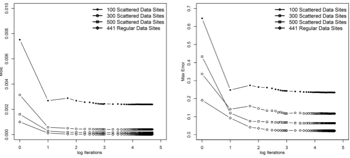
A key issue with the proposed approach is the number of aggregation itera-tions required to produce a reasonable interpolation. Fig. 7 shows the number of aggregation iterations against MSE and Max Error for the Hilbert-Const in-terpolation of Franke’s function. The convergence is largely independent of the number of data-sites and there is little to gain after around 1000 iterations. A similar result has been obtained for Hilbert-Linear interpolation.

Fig. 7: Number of aggregation iterations versus MSE (leftmost graph) and Max Error (rightmost graph). Note the x-axis has a base-10 log scale.

In this section, analysis of interpolating specific functions was considered. In the next section the proposed approach is re-interpreted so that we can reason about it by considering only the location of the data-sites, i.e without the need of a ground truth function to interpolate.

6

Further Analysis

(a) 2D heatmap (b) 3D

Fig. 8: Probability mass function showing the probability that the nearest neigh-bour is the data-site denoted by an×.

the probability that data-sitexiis the nearest neighbour toqj along the Hilbert curve under the Monte Carlo sampling described in the Aggregation Section, i.e.

ˆ

f(q_j) = n

∑

i

pizi (1)

Consider the case where there are only two data-sites, denoted × and ·, located within a region of interest shown in Fig. 8(a) (ignoring the heatmap for the moment). Under Euclidean distance, locations that are closest to the data-site denoted by an×are to the left of the dashed line.

The heatmap represents all the possible query site locations within the region of interest and shows the probability the × data-site is the nearest neighbour under the Monte Carlo sampling, with η = 50,000. Fig. 8(b) shows the same probability mass function but in 3D. It is clear that there is a discontinuity at the peak (corresponding to the× data-site).

Referring back to Equation 1, for the interpolated function ˆf(·) to be con-tinuous, both pi andzi are required to spatially continuous over the region of interest. Assuming that the function to be interpolated is indeed continuous, i.e.

zi is continuous, then pi needs to be continuous. As has been noted, pi is not continuous at data-sites. Hence the interpolated function will not be continuous at data-sites. Note that natural neighbour interpolation also has this issue. The smoothness of probability mass function elsewhere in Fig. 8(b) is consistent with

pi being continuous everywhere apart from at data-sites.

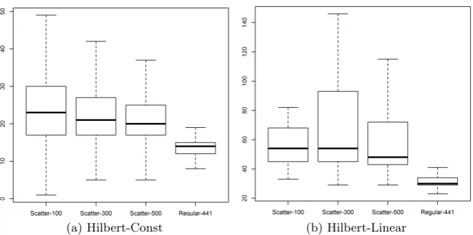
(a) Hilbert-Const (b) Hilbert-Linear

Fig. 9: Number of non zero weighted data-sites for each query location. Hilbert-Linear has more than Hilbert-Const since for linear interpolation uses two data-sites for interpolation whereas constant only requires one.

independent of the increasing number of data-sites. This is a crucial observation for the utility of the proposed approach for large datasets. It suggests that the interpolation is local to the query data-site.

There is one exception, query points near the boundary of the region of interest. Fig. 9 show there is a large variance in the number contributing data-sites per query site. This phenomena is due to the space-filling curve exiting region of interest and entering at some other location along the boundary. This behaviour is not necessarily wrong, it is making the assumption that the function is homogeneous around the boundary. One way to remove this edge effect is to introduce a post-processing step that keeps the closestwcontributing data-sites for each query site near the boundary, wherewis the overall mean.

7

Conclusion and Future Work

The 1D interpolation schemes plugged in to the framework were selected for their simplicity and their amenability to further analysis. However more sophisticated methods could be used. For example basing the interpolation on 1D wavelets [5].

This framework can be extended to perform density estimation by simply replacing the interpolation function with a 1D density estimator. This is possible since the Hilbert curve has the property that it ismeasure preserving, which in the 2D case means that equal lengths along the curve correspond to equal areas. In his context the approach would fit in with the class of Monte Carlo density estimators such as random average shifted histograms [2].

References

1. Bader, M.: Space-Filling Curves: An Introduction with Applications in Scientific Computing, vol. 9. Springer (2012)

2. Bourel, M., Fraiman, R., Ghattas, B.: Random average shifted histograms. Com-putational Statistics & Data Analysis 79, 149–164 (2014)

3. Braun, J., Sambridge, M.: A numerical method for solving partial differential equa-tions on highly irregular evolving grids. Nature 376, 655 – 660 (1995)

4. Chen, H.L., Chang, Y.I.: All-nearest-neighbors finding based on the hilbert curve. Expert Systems with Applications 38(6), 7462–7475 (2011)

5. Lamarque, C.H., Robert, F.: Image analysis using space-filling curves and 1D wavelet bases. Pattern Recognition 29(8), 1309–1322 (1996)

6. Lazzaro, D., Montefusco, L.B.: Radial basis functions for the multivariate interpo-lation of large scattered data sets. Journal of Computational and Applied Mathe-matics 140(1), 521–536 (2002)

7. Ledoux, H., Gold, C.: An efficient natural neighbour interpolation algorithm for geoscientific modelling. In: Developments in Spatial Data Handling, pp. 97–108. Springer (2005)

8. Li, J., Heap, A.D.: Spatial interpolation methods applied in the environmental sciences: A review. Environmental Modelling & Software 53, 173 – 189 (2014) 9. Mari, J.F., Le Ber, F.: Temporal and spatial data mining with second-order hidden

markov models. Soft Computing 10(5), 406–414 (2006)

10. Mennis, J., Guo, D.: Spatial data mining and geographic knowledge discovery. an introduction. Computers, Environment and Urban Systems 33(6), 403 – 408 (2009) 11. Ohashi, O., Torgo, L.: Spatial interpolation using multiple regression. In: 2012 IEEE 12th International Conference on Data Mining. pp. 1044–1049. IEEE (2012) 12. Okabe, A., Boots, B., Sugihara, K., Chiu, S.N.: Spatial tessellations: concepts and

applications of Voronoi diagrams, vol. 501. John Wiley & Sons (2009)

13. Park, S., Linsen, L., Kreylos, O., Owens, J., Hamann, B.: Discrete Sibson inter-polation. Visualization and Computer Graphics, IEEE Transactions on 12(2), 243 –253 (March-April 2006)

14. Sagan, H.: Space-Filling Curves. Springer-Verlag (1994)

15. Skilling, J.: Programming the hilbert curve. In: Bayesian Inference and Maximum Entropy Methods in Science and Engineering: 23rd International Workshop on Bayesian Inference and Maximum Entropy Methods in Science and Engineering. vol. 707, pp. 381–387. AIP Publishing (2004)