Implementation of Two Degree Of Freedom (2DOF) Controller Using Coefficient Diagram Method (CDM) Techniques for Three Tank Interacting System

(1)

Page 90

IMPLEMENTATION OF TWO-DEGREE-OF-FREEDOM (2DOF)

CONTROLLER USING COEFFICIENT DIAGRAM METHOD (CDM)

TECHNIQUES FOR THREE TANK INTERACTING SYSTEM

K. Senthilkumar

1

_{and Dr. D. Angeline Vijula}

2

1

_{PG Scholar, Department of Control and Instrumentation Engineering, Sri Ramakrishna Engineering College,}

Coimbatore, Tamilnadu, India.

2

_{Professor and Head, Department of Control and Instrumentation Engineering, Sri Ramakrishna Engineering}

College, Coimbatore, Tamilnadu, India.

---***---

Abstract – This study presents the design of a

Two-Degree-of-Freedom (2DOF) controller using Coefficient Diagram Method (CDM) techniques for three tank interacting system. By using the Taylor series, the mathematical modeling of nonlinear three tank interacting system is approximated as First Order Plus Dead Time (FOPTD) transfer function. Based on the CDM technique, the parameters of 2DOF controller are designed and implemented in three tank interacting system using MATLAB software. The servo performance of the proposed 2DOF controller using CDM technique control strategy is compared with the conventional PI controller. Finally, the performances of the two controllers are compared and analysed. The simulation results show that the proposed 2DOF controller using CDM technique control strategy is effective and potential for severe nonlinear control problem.

Key Words:

Three Tank Interacting system,

Two-Degree-of-Freedom (2DOF), Coefficient Diagram

Method (CDM), Conventional PI controller.

1. INTRODUCTION

Process industries utilizes three tank interacting system for processing of two different chemical composition streams into a required chemical mixture in the mixing reactor process, with monitoring and controlling of flow rate and level of chemical streams. In most of the chemical plants, level control is extremely important because desired production rates and inventories are achieved through proper control of flow and level. The performance of some processes such as chemical reactors depends critically on the residence time in the

vessel which in turn depends on the level. At this point it is clear that level control is an important control objective. Due to the pronounced non linear nature of several chemical processes, interest in non linear feedback control has been steadily increasing over the last several years [1]. The physical hardware unit of three tank interacting system is shown in the Figure 1.

Fig-1: Physical setup of three tank interacting system

(2)

Page 91

The algebraic design approach namely CDM was developed and introduced by Shunji Manabe in 1998. CDM uses polynomial expressions to represent both the plant and the controller. In this representation, all the equations deal with numerator and denominator polynomials independent from each other and hence the ambiguity that arises due to pole zero cancellations is avoided. In CDM, the characteristic polynomial of the closed loop system is framed using key factors namely stability indices and equivalent time constant. Taking the key factors into account, the coefficients of the controller polynomials are found. The close relation between the conditions embedded via key factors in the characteristic polynomial and the coefficients of the controller polynomials makes CDM technique effective not only for control system design but also for controller parameter tuning [3].

In the present work, an attempt is made to design 2DOF controller using CDM technique for three tank interacting system. The important features of CDM are adaptation of the polynomial representation for the plant and the controller, nonexistence or existence of very small overshoot in the closed loop response, obtaining the characteristic polynomial of the closed loop system efficiently by taking a good balance of stability. This technique leads to good robustness of the control system with uncertainty in the plant parameters. The strength of CDM is simple and can be designed for any plant [4].

The remaining contents of the paper are organized as follows. Section 2 gives the mathematical modeling of three tank interacting system. In section 3, the proposed 2DOF controller using CDM technique is presented. Section 4 gives the design of Conventional PI Controller. Results and discussions are described in section 5. Finally concluding remarks are given in section 6.

2. MATHEMATICAL MODELING OF THREE TANK

INTERACTING SYSTEM

Consider an interacting cylindrical three tank process system, with single input & single output (SISO system). The control objective is to maintain a level (h3) in tank-3 by manipulating the varying inflow rate (q1) of tank-1, shown in the Figure 2.

Fig-2: Schematic diagram three tank interacting system

Where,

 The volumetric flow rate into tank-1 is q1 (cm3/sec)  The volumetric flow rate from tank-1 to tank-2 is

q12 (cm3/sec)

 The volumetric flow rate from tank-2 to tank-3 is q23 (cm3/sec)

 The volumetric flow rate from tank-3 is q4 (cm/sec)  The height of the liquid level in tank-1 is h1 (cm)  The height of the liquid level in tank-2 is h2 (cm)  The height of the liquid level in tank-3 is h3 (cm)  Three tanks (1, 2 and 3) have the same cross

sectional area A1 , A2 and A3 (cm2)

 The cross sectional area of interaction pipes are given by a12 ,a23 and a4 (cm2)

 The valve coefficients of interaction pipes are given by c12 , c23 and c4

According to Mass Balance Equation, Accumulation = Input – Output Adh(t)

dt = qin t − qout t (1)

Applying Mass Balance Equation on Tank-1:

A1 dh1 (t)

dt = q1 t − a12 t . c12 t . 2g(h1− h2) (2)

A2 dh2 t

dt = a12 t . c12 t . 2g h1− h2

− a23 t . c23 t . 2g(h2− h3) (3)

A3 dh3 t

dt = a23 t . c23 t . 2g h2− h3

− a4 t . c4 t . 2gh3 (4)

(3)

Page 92

f h, Q = f hs − Qs + ∂f(h−h_s)

∂h + ∂f(Q−Q_s)

∂Q (5) Linearization using Taylor Series Method on Tank-1: dx1 (t)

dt = 1

A1 Q1 t − T1. x1 t + T1. x2 t (6)

Linearization using Taylor Series Method on Tank-2: dx₂(t)

dt = 1

A2 T1. x1 t − T1 + T2 . x2 t + T2. x3 t (7)

Linearization using Taylor Series Method on Tank-3: dx3 (t)

dt = 1

A3 T2. x2 t − T2 + T3 . x3 t (8)

Where,T1= a

12 g

2 h1− h2

,

T2= a

23 g

2 h2− h3

and

T3= a

4 g

2 h3

; x1 t = h1 t − h1;

x2 t = h2 t − h2andx3 t = h3 t − h3

The operating parameters of the three tank interacting system are given in the following Table 1.

Table-1: Operating parameters of three tank interacting system

PARAMETERS DESCRIPTION VALUES

g Gravitational force

(cm2 /sec)

981

a12 , a23 & a4 Area of pipe (cm2) 3.8 h1s Steady state water

level of tank-1 (cm) 10 h2s Steady state water

level of tank-2 (cm) 7.5 h3s Steady state water

level of tank-3 (cm) 5 A1, A2 & A3 Area of Tank (cm2) 176.71

C12 Valve coefficient of

tank-1 1

tank-2 1

tank-3 0.45

Based on the linearized equations and above operating parameters of three tank interacting system, we obtained the state equation and output equation (State Space Model) of the SISO tank system.

STATE EQUATION: h1

h2 h3

=

−0.3012 0.3012 0

0.3012 −0.6024 0.3012

0 0.3012 −0.3970

h1 h2 h3

+ 0.005680 0

q1 (9)

OUTPUT EQUATION:

y = 0 0 1 h1 h2 h3

+ 0 (10)

Based on the above state space model of the three tank interacting system, we obtain the transfer function of the system by using coding in the MATLAB software.

H3 s

Q1 s =

0.0005133

s3_{+ 1.301 s}2_{+ 0.3587 s+0.008691}

(11)

The FOPDT model of interacting three tank process (SISO System) is approximated using two point methods from actual third order transfer function system. The two point method [4] is used here. The method uses the times that reach 35.3% and 85.3% of the open loop response.

Gp s =

0.0591 e−5s

36.79s+1

(12)

Where,

td = time delay = 5 sec

τ = time constant = 36.79 sec

Kp = proportional gain = 0.0591

3. DESIGN OF 2DOF CONTROLLER USING CDM

TECHNIQUE

3.1 Design concept of CDM Controller:

The block diagram of CDM control system is shown in the Figure 3. In this figure, r is the reference input, y is the system output, u is the controller signal and d is the external disturbance signal. N(s) and D(s) are the numerator and denominator polynomials of the plant transfer function.

(4)

Page 93

A(s) is the forward denominator polynomial, while B(s) and F(s) are the feedback numerator polynomial and reference numerator polynomials of the controller transfer function.

For the given system, the output of the CDM control system is given by,

y = N s F(s) P(s) r +

A s N(s)

P(s) d

(13)

Where, P(s) is the characteristic polynomial of the closed-loop system and defined by,

P s = A s D s + B s N s = ni=0 aisi , ai > 0

(14)

Here, the controller polynomials (A(s) and B(s)) are given as,

A (s) = lisi p

i=0 andB (s) = kisi

q

i=0 (15)

When polynomial F(s) is chosen as

F s =P(s)

N(s) ⎮s = 0

(16)

the overall closed loop transfer function becomes Type-I system. Therefore a good closed-loop response can be achieved.

The design parameters of CDM are the stability indices (γi) and equivalent time constant (τ). The stability indices determine the stability of the system and the transient behavior of the time domain response (with overshoot, without overshoot and oscillations etc.). In addition, they determine the robustness of the system to parameter variations. The equivalent time constant, which is closely related to the bandwidth and it determines the rapidity of the time response. According to Manabe (1998), the design parameters are defined as follows

τ = ts

2.5 ≅ 3

(17)

Where ts is the user specified settling time γi = [2.5 2 2…], where i=1,…., n-1, γ0 = γi = 0 (18)

If necessary, the designer can modify the values of stability indices.

Using the design parameters defined in equation (17) and equation (18), a target characteristic polynomial (Ptarget(s)) is formulated as

Ptarget s = a0 1 γ_i−jj i−1

j=1 (τs)i

n

i=2 + τs + 1

(19)

By substituting the controller polynomials in equation (15) into equation (14), the closed loop characteristic polynomial P(s) are obtained. This polynomial is compared with equation (19) to obtain the coefficients of CDM controller polynomial li, ki, and ai [6].

3.2 Design of CDM based Controller Parameter

for Three Tank Interacting System:

The process considered for this study is three tank interacting system. The mathematical model of three tank interacting system is expressed as polynomial form, given below.

Gp s =

−0.2955 s+0.1182

183 .95s2_{+ 78.58s+2}

(20)

Since CDM is a polynomial-based method, the transfer function of the system is thought to be two independent polynomials (N(s) and D(s)) as shown in Figure 2. These polynomials are,

N(s) = -0.2955s + 0.1182 and D(s) = 183.95s2 _{+ 78.58s + 2 (21)}

The explicit forms of the controller polynomials A(s) and B(s) appearing in the CDM control system structure as shown in Figure 2 are represented by Equation (15). In this work, the controller polynomials are chosen for the step disturbance signal. By considering the equivalent transfer function of the system given in Equation (20), the controller polynomials have forms

A(s) = l2 s2 + l1s and B(s) = k2s2 + k1s + k0 (22)

Where l2, l1, k2, k1 and k0 are controller design parameters. it is considered that there is a step disturbance affecting the system. Thus, let the structure of the controller be chosen with l0 = 0 as follows.

Gc s = B s A s =

k2s2+ k1s+ k0

l2s2+ l1s

(23)

By substituting Equation (21) and Equation (22) in Equation (14), the characteristic polynomial of the control system is obtained as

P(s) = 183.95l2s4 + (78.58l2 + 183.95l1 – 0.2955k2)s3 + (2l2 + 78.58l1 –0.1182k2 – 0.2955k1)s2 + (2l1 + 0.1182k1 – 0.2955k0)s + 0.1182k0 (24)

By substituting the values of the equivalent time constant (τ) and the stability indices (γi) in Equation (19), the target characteristic polynomial is formulated as

Ptarget s = τ4 γ3γ22γ13

s4₊ τ3 γ2γ12

s3₊τ2 γ1 s

2_{+ τs + 1 (25)}

Based on the simulation the user specified sampling time ts is obtained as 109 seconds and calculated time constant τ = 39.20 seconds.

ts = 109 sec and τ = 39.20 sec (26)

By substituting the above value of time constant in Equation (25), we have

(5)

Page 94

By equating the coefficients of the terms of equal power of Equation (24) and Equation (27), the CDM controller parameters (l2, l1, k2, k1 and k0) are computed as follows l1 = 0.4014; l2 = 65.7804; k0 = 8.4602; k1 = 346.0719; and k2 = 4687.67 (28)

The pre-filter (F(s)) are chosen by Equation (16) and calculated as

F(s) = 8.4602 (29)

3.3 Design of 2DOF Controller using CDM

Parameter for Three Tank Interacting System:

[image:5.595.44.276.331.388.2]

The Computation of 2DOF controller with CDM parameters has been calculated here, the standard block diagram given in Figure 3 is reduced as its equivalent block diagram as shown in Figure 4 using block diagram reduction techniques.

Fig-4: Equivalent CDM block diagram From the above Figure 4, the values obtained are F(s)

B(s)=

8.460

4687 .67s2+ 346 .07s+ 8.460 (30) B(s)

A(s)=

4687 .67s2+ 346 .07s+ 8.460

[image:5.595.330.542.389.448.2]

65.780 s2+ 0.401 s (31) Implement the above Equations (30) and (31) in Figure (4), then obtain the desired set point tracking response in the MATLAB simulation. The Simulink model for Two-degree-of-freedom controller with CDM is shown in the Figure 5.

Fig-5: Simulink model for Two-degree-of-freedom controller with CDM

4. DESIGN OF CONVENTIONAL PI CONTROLLER

The PI controller consists of proportional and integral term. The proportional term changes the controller output proportional to the current error value. Large values of proportional term make the system unstable. The Integral term changes the controller output based

on the past values of error. So, the controller attempts to minimize the error by adjusting the controller output. The PI gain values are calculated by using the MATLAB auto tuning algorithm.

u t = Kc e t + 1

T_i e t dt t

0 (32)

The PI Tuner allows to achieve a good balance between performance and robustness for either one or two-degree-of-freedom PI controllers. PI Tuner is used to tune PI gains automatically in a Simulink model containing a PI Controller or PI Controller (2DOF) block. The PI Tuner considers as the plant all blocks in the loop between the PI Controller block output and input. The blocks in the plant can include nonlinearities. Because automatic tuning requires a linear model, the PI Tuner computes a linearized approximation of the plant in the model. This linearized model is an approximation to a nonlinear system, which is generally valid in a small region around a given operating point of the system.

The obtained gain values of PI controller based on the auto tune method is proportional gain Kp = 2.2093 and integral gain Ki = 0.4504. The Simulink model for conventional PI controller is shown in Figure 6.

Fig-6: Simulink model for conventional PI controller

5. RESULTS AND DISCUSSION

5.1 Closed Loop Response of 2DOF Controller

using CDM:

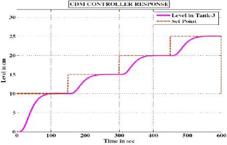
[image:5.595.38.281.551.629.2]

The closed loop response obtained using the Two-degree-of-freedom controller (2DOF) with CDM is shown in the Figure 7, based on the controller design.

[image:5.595.324.548.592.735.2]

(6)

Page 95

5.2 Closed Loop Response of Conventional PI

Controller:

The closed loop response obtained using Conventional PI controller is shown in the Figure 8, based on the controller design.

Fig-8: Response of Conventional PI controller

5.3 Comparative Closed Loop Response:

The comparative closed loop response of proposed controller is shown in the Figure 9, based on the controller design.

Fig-9: Comparative closed loop response

Based on the above response of the 2DOF controller using CDM and Conventional PI controller, the performance metrics are calculated and given in the below Table 2.

Table-2: Comparative performance metrics of 2DOF using CDM and Conventional PI controller:

Performance

Metrics Conventional PI Controller

2DOF Controller using CDM

Rise Time (sec) 90 100

Settling Time (sec) 470 110

Peak Time (sec) 135 120

Peak Overshoot (%) 16 0

Integral Absolute

Error (IAE) 1258 852

From the Table 2, the comparative analysis of controller performance based on the rise time, settling time, peak time, peak overshoot and integral absolute error of time domain response of the proposed system.

By comparing the performance of 2DOF controller using CDM with conventional PI controller, the 2DOF controller using CDM has better response because it does not contain overshoot in output response and also the IAE value is 852 which is low when compared to the value of Conventional PI Controller. Therefore 2DOF controller using CDM has better, no overshoot and robust response in output, which is verified in the simulation result.

6. CONCLUSION

The three tank interacting system is a highly non-linear process because of the interaction between the tanks. The controlling of nonlinear process is a challenging task. In this paper, the linearized model of three tank interacting system was obtained.

The 2DOF controller using CDM technique and Conventional PI controller are designed and simulated using MATLAB. From the results, it is proved that the 2DOF controller using CDM responses are fastest according to rise time and have smallest settling time with no peak overshoot. Finally, the proposed 2DOF controller using CDM control strategy can be applied to any hybrid tank interacting processes to obtain the improved closed loop system performance under practical environment.

REFERENCES

[1] P.K. Bhaba (2009), “Real Time Implementation of A New CDM-PI Control Scheme in A Conical Tank

Liquid Level Maintaining System”, Journal of Applied

(7)

Page 96

[2] M. Chidambaram, B.C. Reddy, and D.M.K. Al-Gobaisi (1997), “Design of robust SISO PI controllers for a

MSF desalination plant”, J. Desalination, No.109,

pp.109 -119.

[3] P.K. Bhaba, and S. Somasundaram (2011), “Design and Real Time Implementation of CDM-PI Control

System in a Conical Tank Liquid Level Process”,

Sensors & Transducers Journal, Vol.133, No.10, pp. 53-63.

[4] S.E. Hamamci, M. Koksal, & S. Manabe (2002), “On the control of some nonlinear systems with the

Coefficient Diagram Method”, 4th Asian Control

Conference, Singapore.

[5] K.R. Sundaresan and P.R. Krishnaswamy (1978),

“Estimation of Time Delay Time Constant Parameters

in Time, Frequency, and Laplace Domains”, The

Canadian Journal of Chemical Engineering, Vol.56, No.2, pp.257-262.

[6] B. Meenakshipriya, K. Saravana, K. Krishnamurthy and P.K.Bhabha (2012), “Design and implementation of CDM-PI control strategy in pH neutralization

system”, Asian Journal of Scientific Research, Vol.5,

No.3, pp 78-92.

[7] K. Kalpana and B. Meenakshipriya (2014), “Design of Coefficient Diagram method (CDM) based PID controller for Double Interacting Unstable System”, IEEE, pp. 189-193.

[8] Erkan IMAL (2009), “CDM based controller design

for nonlinear heat exchanger process”, Turkey

Journal of Electrical Engineering & Computer Science, Vol.17, No.2, pp.143-161.

[9] S.E. Hamamci and M. Koksal (2003), “Robust Controller Design for TITO Processes with Coefficient

Diagram Method”, IEEE, pp.1431-1436.

[10]Arjin Numsomran, Tianchai Suksri and Maitree Thumma (2007), “Design of 2-DOF PI Controller with

Decoupling for Coupled-Tank Process”, International

Conference on Control, Automation and Systems, pp.339-344.

[11]N. Kanagasabai and N. Jaya (2014), “Design of Multiloop Controller for Three Tank Process using

CDM Techniques”, IJSC, Vol.5, No.2, pp.11-20.

[12]Shunji Manabe (2002), “Brief Tutorial and Survey of

Coefficient Diagram Method”, The 4th Asian control

Conference, pp.1161-1166.

[13]B. Roffel and B.H. Betlem (2004), “Advanced

Practical Process Control”, Springer (India) Private

Limited publication, Indian Edition.

[14]Wayne Bequette B. (2003), “Process control

modeling, design and simulation”, PHI Learning

Private Limited publication, Indian Edition.

[15]William L. Luyben (1990), “Process Modelling,

Simulation, and Control for Chemical Engineers”,

McGraw-Hill publication, Singapore, International Edition.

BIOGRAPHIES

K. Senthilkumar received his Bachelor’s Degree in Instrumentation

and Control Engineering from

Tamilnadu College of Engineering in 2010. He is currently pursuing Master’s Degree in Control and Instrumentation Engineering from Sri Ramakrishna Engineering College. He has 2 years 7 months of work experience in Wind Research Department in Gamesa Wind Turbines Pvt. Ltd. Chennai. His research interests are Renewable Energy Resources, Process Control and

Control Systems.

Dr. D. Angeline Vijula received her Master’s Degree in Applied Electronics from P.S.G College of Technology in 2006. She received her Bachelor’s Degree in Instrumentation and Control Engineering (ICE) from Madurai Kamaraj University in 1994. Her research interests are Multivariable

Control, Process Control

Instrumentation and Industrial