Financial Development, Shocks, and Growth Volatility

Munich Personal RePEc Archive

Financial Development, Shocks, and

Growth Volatility

Mallick, Debdulal

Deakin University

October 2009

Online at

https://mpra.ub.uni-muenchen.de/17799/

Financial Development, Shocks, and Growth Volatility

Debdulal Mallick*

School of Accounting, Economics and Finance Deakin University

Burwood, VIC 3125 Australia

Phone: (61 3) 92517808 Fax: (61 3) 92446283 Email: dmallic@deakin.edu.au

This Draft: October 2009

* I acknowledge helpful comments from Robert Chirinko, Arusha Cooray, Daniel Levy, Devashish Mitra, Paresh Narayan, and Randy Silvers and participants at 2009

Australasian Econometric Society Meeting. Partial financial support from Deakin

University’s Faculty of Business and Law Developing Researcher Grant is

Financial Development, Shocks and Growth Volatility

Abstract

This paper argues that studying the effect of financial development and shocks on

aggregate growth volatility will not be informative because they affect growth volatility

through its different components. Volatility declines either a consequence of a change in

the nature of shocks or a change in how the economy reacts to shocks. If two economies

differ only in terms of volatility of shocks experienced, the GDP growth spectrum of one

economy will lie proportionately below that of another at all frequency ranges so that

both business cycle and long-run variances will be lower. Conversely, if change in

volatility is due to propagation mechanism such as financial development, a country

having developed financial markets will have disproportionately lower variance at the

business cycle than at other frequencies relative to that of a country having less

developed financial markets. Therefore, the variance at only the business cycle frequency

range will be influenced by financial development. The novelty of this paper is that

different components of growth volatility are extracted using spectral method.

Empirical evidence provides qualified support for both hypotheses. Higher private

credit, which is used as proxy of financial development, dampens business cycle

volatility but not the long-run volatility. Shocks, as measured by changes in the terms of

trade, affect both business cycle and long-run volatility negatively. These results are

robust to alternative market-based measure of financial development, and corrections for

reverse causality. These results have important implications for growth theory as they

shed lights on the factors causing permanent and transitory deviations from the steady

state.

JEL Classification codes: C21, C22, E32, E44, O16, O50

Financial Development, Shocks and Growth Volatility

I. Introduction

Growth models focus on the trend growth and a large body of literature has

studied the role of the financial development in economic growth.1 Business cycle

volatility is related to financial development through several channels including the flow

of information and the enforcement of contracts. Shocks, on the other hand, generate and

magnify the business cycle volatility and also affect the long-run trend growth that

depends on the shock persistence. There are several models that try to bridge growth and

business cycle models and explain the role of financial development and shocks in

growth volatility (Aghion et al., 2007, and papers cited therein). There is also a nascent

literature that empirically investigates the role of financial development in growth

volatility but without making any distinction between its long-run and business cycle

components. These studies use the standard deviation of the growth rate of per capita real

GDP as the measure of volatility.

In this paper we argue and show that financial development and shocks affect

total volatility through its different components. Specifically, we show that financial

development impacts only on the business cycle component of volatility while shocks

impact on both the long-run and business cycle components, and therefore on total

volatility. In other words, volatility caused by shocks is more persistent than that caused

by financial underdevelopment.2 This paper can be considered as an attempt to

investigate the bridge between the two approaches mentioned above. The novelty of this

paper is that it employs spectral method to extract business cycle and long-run

components of the variance of the growth rate of real GDP per capita. This investigation

has also important implications for growth theory. Previous studies do not distinguish the

factors that cause permanent and transitory deviations from the steady state growth rate.

1

Levine (1997) provides an excellent discussion. 2

This paper sheds some lights on this issue by investigating two important factors—

financial development and shocks.

Assuming that the output growth series is covariance stationary, its variance can

be expressed as the integral of the spectrum of the series across all frequencies,

  

   . Therefore, a country with lower growth variance would have a spectrum

lying below the one for the country with higher growth variance. It does not necessarily

mean that the spectrum will lay below at all frequency ranges; the area under the

spectrum will be smaller. Distribution of the two spectra across different frequency

ranges is very informative in explaining the relative volatility at different frequency

ranges (Ahmed et al., 2004, p. 825).

Any stochastic model of the economy can be thought of a combination of some

shocks and a propagation mechanism. Output growth volatility declines either as a

consequence of a change in the nature of shocks or as a change in the propagation

mechanism, i.e., a change in how the economy reacts to shocks, or a combination of both.

If two economies differ only in terms of volatility of shocks experienced, the GDP

growth spectrum of one economy will lie proportionately below that of another at all

frequency ranges. The reason is that a covariance-stationary series, such as output

growth, can be expressed as an infinite moving-average (MA) process whose spectrum is

proportional to the innovation variance. Therefore, the lower volatility of shocks can be

interpreted as a lower innovation variance with the same MA coefficients for two

economies. Given that a particular component of the variance is the integral of the

spectrum over the respective frequency ranges, both the long-run and business cycle

components of the variance will be lower for the country experiencing lower volatility of

shocks.

Conversely, if change in volatility is solely due to change in propagation

mechanism, such as financial development, this would be manifested in the contour of

the spectrum (Ahmed, et al., 2004, p. 824). One would expect that, ceteris paribus, the country having developed financial markets will have disproportionately lower variance

at the business cycle than at other frequencies relative to that of a country having less

developed financial markets. Therefore, the variance at the business cycle frequency

better inventory management that smooth output in the short-run is mainly responsible

for lower volatility, variance will be lower primarily at relatively high frequencies.

Measurement errors would also be reflected in the high frequency range. Finally, if a

lower volatility is due to a combination of changes in both shocks and propagation

mechanism, one spectrum will lie below another disproportionately at some frequency

range depending on the relative importance of the factors.

The above econometric argument can also be supplemented by predictions of

growth models. The main argument is that shocks generate long-run volatility but

financial development does not. The real business cycle (RBC) models cannot explain

persistence volatility unless shocks are very volatile and persistent. In endogenous

growth models, shocks generate persistent volatility. For example, in Fatás (2002),

expected profitability of innovation depends on aggregate demand, and negative shocks

to aggregate demand reduce the incentive to innovate. When the economy gets out of

recession, innovation is permanently lower and therefore, output remains at a

permanently low level. Economic downturns also impact negatively on the amount of

learning by doing that permanently lowers the steady state growth rate (Stadler, 1986;

1990).

There are several models that explain the role of financial development in

business cycle volatility but long-run volatility does not occur in standard situations. The

best example can be Aghion and Banerjee (2005) where long-run volatility is a remote

possibility for intermediate level of financial development. They show that financial

underdevelopment interacts with interest rate (or real exchange rate in open economy) to

generate volatility but volatility can be persistent (in the sense that an economy exhibits

limit cycles) only in the countries at the medium level of financial development.

Investments and borrowing are higher in a boom that leads to higher interest rate. But

higher interest rate also creates a pecuniary externality as it increases the debt burden of

all entrepreneurs, which slows down growth of entrepreneur’s wealth and investment

capacity. At some point, investment capacity falls below total savings, the economy

enters recession and interest rate will eventually fall. The process will then revert to a

boom. But only countries at intermediate level of financial development may experience

their retained earnings for investment. On the other hand, financially developed countries

will not also experience long-run volatility because firms can invest up to the expected

net present value of their project since they face no credit constraints.

Based on the above discussions, this paper aims to test two hypotheses. First, a

country with developed financial markets will experience lower business cycle

component of growth volatility but the long-run component will not be affected by such

development. The effect on total volatility will, therefore, depend on the share of the

business cycle component in total volatility. Second, a country experiencing lower shocks

will have both lower business cycle and long-run components of volatility and, therefore,

lower total volatility. Our measure of financial development is the private sector credit by

bank and other financial institutions as a percentage of GDP. We also check the

robustness using an alternative measure—value of total stock market capitalization as a

percentage of GDP. Both measures are standard in the literature. We use changes in the

terms of trade (TOT) defined as the ratio of export prices to import prices as a proxy

measure of shocks, which is considered as exogenous to a country.

Empirical evidence provides qualified support for our hypotheses. After

controlling for country specific fixed factors and the effects of possible outliers, we find,

in a sample of 79 countries for the period 1980-2004, that higher private credit dampens

the business cycle component of volatility but not the long-run component, while a TOT

deterioration (improvement) magnifies (dampens) both business cycle and long-run

components of volatility. The role of higher private credit in reducing volatility is not

found to be important for the high income countries when examined at different stages of

economic development. However, when we construct a two-period panel only for

selected OECD countries for which longer period of data are available, we find that

higher private credit reduces business cycle volatility for these countries as well. When

private credit is replaced by value of stock market capitalization, we find a robust

negative effect only for the low-income countries. All results are robust to corrections for

reverse causality.

The rest of the paper is organized as follows. Section II briefly discusses different

channels through which financial development dampens growth volatility, reviews

components. We discuss estimation of different components of volatility in the frequency

domain, data and summary statistics at the cross-country level in section III. In section

IV, we present our findings. Finally, section V concludes.

II. Related literature and motivation

The existing literature describes several routes through which financial

development and shocks might impact on volatility.

Developed financial markets and institutions lessen separation between savers and

investors and facilitate diversification which has implications for growth volatility. In

Aghion et al. (1999) savings exceed investment during periods of slow growth resulting

in low demand for savings and therefore low equilibrium interest rates, which in turn

implies that investors can retain large portion of their profits and expand investment. This

process continues until investment increases sufficiently to put upward pressure on

interest rates. Then the process is reversed taking the economy back to a period of slower

growth. The higher the degree of separation between savers and investors, the larger is

the growth volatility. Acemoglu and Zilibotti (1997) argue that in the early stages of

development indivisibility of investment limits the degree of diversification of

idiosyncratic risk that discourages investment in risky projects which are more

productive. This slows down capital accumulation and introduces large growth volatility.

However, Koren and Tenreyro (2007) did not find support that low income countries

invest in safe projects; rather, these countries’ investment is concentrated in more volatile

sectors.

Financial development also reduces volatility by reducing cost of acquiring

information and improving risk management. Underdeveloped financial markets are

characterized by imperfect information and costly enforcement of contracts that interfere

with smooth functioning of the financial market. Bernanke and Gertler (1995) and

Bernanke et al. (1998) argue the balanced sheet (or net worth) channel of the firm in

mitigating business cycle volatility as imperfect information and costly enforcement of

contracts create ―external finance premium‖ that is a wedge between the cost of external

funds and the opportunity cost of internal funds. Tighter monetary policy exacerbates the

problem will be more pronounced in the financially underdeveloped countries where

―external finance premium‖ is greater. Greenwald and Stiglitz (1993) also develop

models in which developed financial markets dampen volatility by reducing information.

In Aizenman and Powell (2003) a weak legal system interacts with high costs for

information verification leading to a first-order effect of volatility on production,

employment and welfare. Their calibration illustrates that a 1% increase in the coefficient

of variation of productivity shocks would reduce welfare by more than 1%. However,

these are not models of persistent business cycle.

Aghion et al. (2007) try to bridge the apparent disjoint between long-run growth

and business cycles models. In their model the share of long-term investment is

countercyclical when the capital market is perfect but becomes procyclical with an

imperfect capital market. Since long-term investment enhances productivity more than

short-term investment, this implies that the cyclical behavior of the composition of

investment mitigates fluctuations when financial markets are perfect, but amplifies them

when credit constraints are sufficiently tight.

There are several studies that empirically investigate the role of financial

development and shocks in growth volatility with mixed support. Easterly et al. (2002)

find that financial development (as measured by private credit to GDP) lowers growth

volatility but in a nonlinear fashion. Financial development reduces volatility up to a

point, but too much private credit can increase volatility. Kunieda (2008) also finds a

nonlinear relationship in thatfinancial development has a hump-shaped effect on growth

volatility. In early stages of financial development, growth rates are less volatile. As the

financial sector develops, an economy becomes highly volatile but becomes less volatile

once again as financial sector matures. Lopez and Spiegel (2002), Denizer et al. (2002),

Silva (2002), and Tharavanij (2007) also confirm a negative relationship between

financial development and growth volatility.

Raddatz (2006) examines US industry level data and finds that financial

development leads to a comparatively larger reduction in the volatility of output in

sectors with high liquidity needs. Phumiwasana (2003)finds evidence that bank-based

volatility among developing countries. However, Silva (2002) finds that bank-based or

market-based financial structure is unimportant in explaining growth volatility.

On the other hand, Tiryaki (2003) and Beck et al. (2006) do not a find relationship

between financial development and growth volatility. Acemoglu et al. (2003) suggest that

distortionary macroeconomic policies are symptoms of underlying institutional problems

rather than main causes of economic volatility. They find thatfinancial aspects become

insignificant for explaining volatility once the effect of institutions are controlled. These

results contrast the mechanisms behind the difference in cross-country growth volatility

explained above.

Beck et al. (2006) investigate the channels through which financial development

potentially affects growth volatility. They find inflation volatility magnifies growth

volatility in countries with low level of financial development but no effect in the

countries with better financial system. They also find weak evidence for a dampening

effect of financial intermediary development on the impact of TOT volatility. Aghion et

al. (2007) use a panel data of 21 OECD countries over the 1960-2000 period and find that

the impact of commodity price shocks on the long-run investment (share of structural

investment is their proxy) is more negative in countries with lower private credit. In

contrast, they find no such effect in the case of overall investment rate.

The literature discussed above invariably uses the standard deviation of the per

capita GDP growth as the measure of volatility3 without making any distinction between

its different components. In the following, we argue that this aggregate measure of

volatility is not informative because financial development and shocks impact on total

volatility through its different components.

Assuming that the output growth series is covariance stationary, its variance can

be expressed as the integral of the spectrum of the series, g( ) , across all frequencies

  

   . A country with lower growth variance would have a spectrum lying below

the one for the country with higher growth variance. It does not necessarily mean that the

spectrum will lay below at all frequency ranges; the area under the spectrum will be

smaller. Distribution of the two spectra across different frequency ranges provides useful

3

information about the relative volatility at different frequency ranges. Ahmed et al.

(2004, p. 825) exploits this information to explain the reduction in different components

of volatility of US GDP growth and inflation for two distinct periods, and the relative

importance of improved monetary policy, exogenous shocks and improved inventory

practices in explaining the reduced volatility. This argument can be extended to explain

varying degree of growth volatility at the cross-country level.4

To understand this, suppose that two countries experience different magnitude of

the volatility of shocks; otherwise, they are similar in terms of their structural features.

Then the spectra of the output growth for the two countries will be of similar shape but

the spectrum of the country experiencing lower volatility of shocks will lay

proportionately below the other at all frequency ranges. This can be explained by Wold’s

theorem, which suggests that output growth, assuming it as covariance-stationary, can be

expressed as an infinite moving-average (MA) process. Since the spectrum of any MA

series is proportional to its innovation variance, the country experiencing lower volatility

of shocks will have lower innovation variance than the other but the MA coefficients will

be the same. Given that a particular component of the variance is the integral of the

spectrum over the respective frequency ranges, all components of the variance will be

lower for the country experiencing lower volatility of shocks. This hypothesis can be

analyzed more precisely using the concept of the normalized spectrum, h( ) g( ) / 2, that indicates the fraction of the total variance, 2, occurring at each frequency. The normalized spectrum is invariant to the magnitude of the innovation variance because

both g( ) and 2 are proportional to the innovation variance. Therefore, the two normalized spectra will be the same.

The argument that shocks generate long-run volatility can also be explained by

endogenous growth theory. For example, in Fatás (2002) optimal research depends on the

expected profitability of innovation (or imitation) which is a function of aggregate

demand. Negative shocks to aggregate demand reduce the incentive to innovate and as a

result when the economy recovers from recession output does not revert to the trend

rather remains at a permanent low level. In Stadler (1986, 1990) economic downturns

4

impact negatively on the amount of learning by doing that also generate persistence

fluctuations. In Kiyotaki and Moore (1997), a negative shock to profit decreases

investment which in turn reduces the price of collateral. This increases borrowing

constraints on investors thus deteriorating investment capacity which amplifies the

negative shock on profit. A negative serial correlation in aggregate output is thus

generated.

In contrast, if the structures of the two economies differ, the spectrum of the

low-volatility country will lie below disproportionately at the business cycle and higher

frequencies. For example, if the lower variance is due mainly to better business practices

such as better inventory management that smooth output on a quarter-by-quarter basis,

variance will be lower primarily at relatively high frequencies. Measurement errors

would also be reflected in these frequencies. If financial development dampens business

cycle fluctuations, as we have discussed above, one would expect that a country having

developed financial markets will have its spectrum disproportionately lower at the

business cycle than at other frequencies relative to that of a country having less

developed financial markets. Therefore, a country with developed financial markets will

have lower business cycle component of the variance than another.

Financial development impacts on long-run growth by reducing information and

transaction costs, which in turn influences saving and investment decisions and

technological innovation (Levine, 1997, p. 689) but its effect on long-run volatility is not

clear. Aghion and Banerjee (2005) develop a model that is capable of generating

endogenous volatility in an economy with credit constraints but long-run volatility can be

a possibility only for countries at the intermediate level of financial development. The

basic mechanism in their model is the interaction of credit constraints and endogenous

changes in the interest rate. Investments and borrowing are higher in a boom that leads to

higher interest rate. But higher interest rate also creates a pecuniary externality as it

increases the debt burden of all entrepreneurs, which slows down growth of

entrepreneur’s wealth and investment capacity. At some point, investment capacity falls

below total savings and the economy enters recession and interest rate will decrease. The

process will then revert to a boom. However, in a highly underdeveloped country

financially developed countries firms face no credit constraints and thus can invest up to

the expected net present value of their project. Therefore, financially developed or

underdeveloped countries will not experience long-run volatility leaving vulnerable the

countries at the intermediate level of financial development. This result also holds in the

context of open economy where the relevant price is the real exchange.

Finally, if a lower volatility is due to a combination of changes in both shocks and

propagation mechanism, one spectrum will lie below another disproportionately at some

frequency range depending on the relative importance of these two.

The above motivation allows us to test the following two hypotheses:

1. Financial development affects only the business cycle component of volatility and

therefore, the effect on total volatility depends on the relative magnitude of its

business cycle component, and

2. Shocks affect both the long-run and business cycle components of volatility and

therefore, total volatility.

III. Volatility at the cross-country level

In this section, we briefly explain the spectral method that is employed to extract

variance at different frequency range. We then present the summary statistics of different

variance components.

III.A Estimation in the frequency domain

The variance of output growth can be expressed as the integral of the spectrum of

this series, g( ) , across all frequencies      . The spectrum is symmetric around zero so that only the frequency range 0   becomes relevant. The novelty of spectral method is that it provides a simple yet elegant way to decompose the total

variance into different components. For example, the long-run component of the variance

will be the integral of the spectrum over the long-run frequency range.5 The business

5

cycle and short-run components can also be extracted in a similar way by integrating the

spectrum over the relevant frequency ranges. The sum of the three variance

components—long-run, business cycle, and short-run—add to the total variance of the

series. It is important to note that any variance component is orthogonal to other

components because the covariance between spectral estimates at different frequencies is

zero.

Suppose, x_t is a covariance-stationary series. The periodogram, which is the

sample analog of the spectrum, is given by:

1 1

0

( 1) 1

1 1

ˆ ˆ ˆ

ˆ( ) 2 cos( )

2 2

T T

j i j j

j T j

g   e    j

            _  _  





autocovariance given by

1

1

ˆ ( )( )

T j

t t j

t j

x x x x T

 _

 





is the sample mean given by

1 1 T t t x x T 





for the frequency range ( ₁, ₂) is given by:

2

1

1 0

2 1 2 1

1 2

1

sin( ) sin( ) 2

ˆ_{( , ) 2 ˆ( ) ˆ} T _ˆ j j

j j

G g d

j                  







variance of the series x_t attributed to the frequency range ₁   ₂. The frequency, , is inversely related to periodicity or cycle length according to p2 / . The frequency ranges of the long-run, business cycle and short-run are given respectively, by 0  ₁,

1 2

    , and ₂    , where values of ₁and ₂ for annual series are chosen to

be 0.786 and 2.09, respectively. These cut-off frequencies are chosen following modern

business cycle literature in that the long-run corresponds to cycles of 8 years or longer,

and the business cycle corresponds to cycles of 3 to 8 years (Baxter and King, 1999).

Therefore, low frequency is related to long-run7 and high frequency is related to

short-run.

6

Variance of x_t is given by 2

1 1 ( ) 1 T t t x x T  





0

ˆ

 because of different

denominators in the two formulas. 7

The periodogram is an asymptotically unbiased estimate of the spectrum

(Priestley, 1981; p.693). But this is inconsistent because the variance of gˆ( ) does not tend to zero as T tends to infinity (Priestley, 1981, p. 432). The reason is that although

ˆ( )

g  involves T sample autocovariances and the variance of each is of order (1/T), the combined effect of the T terms produces a variance of order 1. One way to reduce the variance is to specify a ―spectral window‖, i.e. truncating the periodogram at some

pointM (T 1). We use Bartlett’s window that assigns linearly decreasing weights to

the autocovariances in the neighborhood of frequency considered and zero thereafter. The

number of ordinates, M, is set using the rule M 2 T (Levy and Dezhbakhsh, 2003, p. 1527).8

III.B Data and Descriptive statistics

Growth rate is calculated by taking the first-difference of the log of real per capita

GDP.9 Calculation of the growth variance requires collapsing several years of GDP

growth data. Data on private credit are not available for many countries for a long period.

Given that data come from different sources, we choose the time period 1980-2004 for

the analysis so that GDP and private credit data are available for relatively longer period

for a good number of countries. There are 116 such countries among which, according to

the World Bank classification, there are 39, 50 and 27 low income, middle income and

high income countries respectively. However, data for the control variables used in the

regressions are not available for many countries for that period especially for many

developing countries; therefore, the sample size reduces to 79 countries for which data

for all variables are available (29, 32 and 18 low, middle and high income countries

respectively). Appendix A.1 provides description of all variables, their sources, and time

periods. For several OECD countries, all data are available for a longer period of time.

8

However, Engle (1974, p.3) and Priestly (1981, p. 471) argued that the integrated periodogram is consistent, not because it approaches its spectral value at each frequency, but because the sum (integral) of the periodogram over all frequencies approaches the sum (integral) of the spectral values, which is the variance attributed to frequency ranges. Priestly (1981, p. 483) mentions that both approaches—with and without spectral window—are equivalent as far as their asymptotic sampling properties are concerned. 9

We split the sample period into two intervals—1960-1979 and 1980-2004—to construct a

two period panel for this set of countries.10

Insert Table 1 here

Table 1 reports descriptive statistics of different components of the variance of

GDP growth and their relative shares for 116 countries (variances for all sample countries

are listed in Appendices A.2-A.4). Mean total variance is decreasing with income level. It

is 32.9, 26.7 and 9.6 for the low, middle and high income countries, respectively. The

mean value of business cycle component of the variance follows a similar pattern (13.5,

11.1 and 3.7, respectively). The mean value of long-run component is the same in the

low and middle income countries at 8.3, while it is almost half in the high income

countries. Note that the long-run component of the variance is one way of representing

the degree of shock persistence (Levy and Dezhbakhsh, 2003, p. 1500-01). This then

implies no difference in shock persistence between the low and middle income countries

but the high income countries are about half shock persistent than other countries. The

high income countries include both OECD and non-OECD countries. For the 20 OECD

countries (column 6), the mean value of the variance at each frequency range is lower

than that for all high income countries implying higher variance for the non-OECD high

income countries.

However, another pattern emerges if we examine the share of different variance

components. For example, the mean share of the long-run component is increasing while

the mean share of the short-run component is decreasing with income level. The mean

share of the business cycle component is almost the same for low and middle income

countries (0.42 vs. 0.41) and is slightly lower for the high income countries (0.39). This

finding contrasts Levy and Dezhbakhsh (2003), who find a statistically significant

positive relationship between income level and the share of the business cycle component

of the variance (their Table 6 in p. 1519). Their sample period (1950-1994) and set of

10

countries are different from ours. To compare their results with ours, we compute the

shares for the same set of countries as Levy and Dezhbakhsh for the period 1960-2004

and report the results in Table 2.

Insert Table 2 here

We find that mean share of the business cycle component is marginally increasing

with income level. However, for this set of countries, total variance and also its long-run

and business cycle components are larger for the middle income than low income

countries. This implies that results may be driven by the choice of sample countries and

time period because Levy and Dezhbakhsh sample period excludes more recent crises

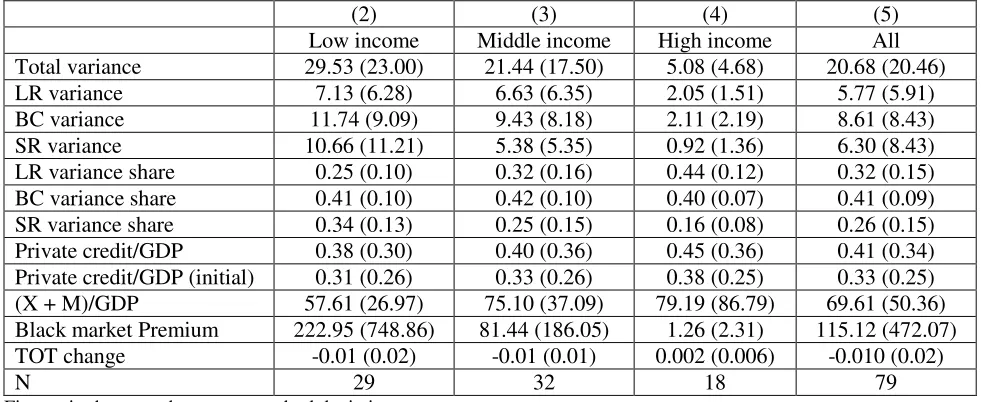
including the East Asian one. We therefore also report the statistics of the 79 countries

included in the regressions (Table 3). Results follow similar patterns in our two samples

(116 countries vs. 79 countries) with the only exception that mean shock persistence

(long-run component of the variance) is now slightly lower in the middle income than

low income countries. It is also evident that in both samples the business cycle

component of the variance dominates in the cases of low and middle income countries,

while it is the long-run component that dominates in the case of high income countries.

On the other hand, in Levy and Dezhbakhsh (2003) sample, the business cycle

component dominates in the case of all income categories.

Insert Table 3 here

There is also a difference in the mean private credit to GDP ratio (which is the

time series average for each country for the 1980-2004 period) in the two samples. In the

sample of 116 countries, the mean is the lowest for the middle income countries (0.38),

while in the reduced sample of 79 countries it is clearly increasing with the income level.

In the latter sample the mean values are 0.38, 0.40 and 0.45 for the low, middle and high

income countries, respectively. The same applies to the initial mean value of private

on average experience negative TOT shocks, while the high income countries

experienced positive TOT shocks.

IV. Empirical analysis

IV.A Estimation method

We follow a simple estimation method in line with other kindred studies in which

we regress long-run and business cycle components of the volatility of the growth rate of

per capita real GDP on financial development, shocks and other variables related to the

growth variances. The equations we estimate are as follows:

_ _i _ _{i i i i}

GrVol bc const  fin dev   shock γX  --- (1)

_ i _ i i i i

GrVol lr const  fin dev   shock γX  --- (2)

_ _i _ _{i i i i}

GrVol total const  fin dev   shock γX  --- (3)

Here, GrVol bc_ _i, GrVol lr_ _i, and GrVol total_ _i are the business cycle, long-run, and

the total volatility of the growth rate of real per capita GDP in country i, respectively. We first calculate variance (and its components) using spectral method, and then take the

square root to calculate volatility. This has been done because in the literature the

standard deviation is used as the measure of volatility. As a measure of financial

development ( fin dev_ _i), we use (log) the value of credit disbursed to the private sector

by banks and other financial institutions relative to GDP. It is preferred to other measures

of financial development because it excludes credit extended to the public sector and

funds provided from central or development banks (Aghion, 2007, p. 17). As a part of

robustness checks, we also use an alternative market-based measure—the value of stock

market capitalization relative to GDP. Our proxy for the shock variable is the change in

the terms of trade (TOT) defined as the ratio of export prices to import prices.

The TOT is exogenous to a country and, therefore, a change in TOT can be considered as

Other controls (X_i) include (log) the initial level of per capital real GDP, the

initial high school enrolment rate that is intended to account for human capital, black

market premium on foreign exchange that accounts for the market distortions, openness

measured as the sum of exports and imports as a percentage GDP, and ―polity score‖,

which is used as a proxy for institutions. All the variables in X_i (excluding the initial

values) are averaged over the period 1980-2004. The institution variable is intended to

isolate the effect of financial development from other institutional characteristics (Aghion

et. al., 2007, p. 19). Acemoglu et al. (2003) suggest that distortionary macroeconomic

policies are symptoms of underlying institutional problems rather than main causes of

economic volatility. They find thatfinancial aspects become insignificant for explaining

volatility once the effect of institutions are controlled. Mobarak (2005) also finds that

higher levels of democracy and diversification lower volatility. The ―polity score‖ is an

index taken from Polity-IV dataset that captures the regime authority spectrum on a

21-point scale ranging from -10 (hereditary monarchy) to +10 (consolidated democracy). It

examines concomitant qualities of democratic and autocratic authority in governing

institutions, rather than discreet and mutually exclusive forms of governance.

We also include country characteristics such as latitude, dummies for tropical and

landlocked countries and legal origins. Some regions, such as East Asia and Latin

America, have experienced severe economic crises than others and crises in some regions

are also more frequent. In order to control for the effect of the outliers, we also include

regional dummies.

IV.B Benchmark Results

Although the dependent variables are ―generated‖, measurement errors are

unlikely to influence our results for two reasons. First, the effect of measurement errors in

the dependent variable is not statistically serious in the classical sense as these are

absorbed into the residual term. Second, measurement errors corrupt estimates at the high

frequency range. We focus on the long-run and business cycle components of the

variance that exclude high frequency components. However, total variance, as in other

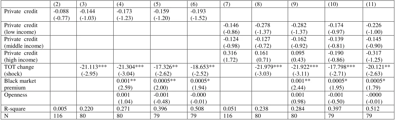
Insert Table 4 here

Table 4 reports the results for equation (1) where business cycle volatility is the

dependent variable and credit to the private sector relative to GDP is the measure of

financial development. Columns 2-6 report results for various combinations of the

explanatory variables. In all regressions, the coefficient of private credit is negative and

statistically significant at least at 10% level. The significance level increases to 5% when

country specific fixed factors and regional dummies are controlled for. The magnitude of

the coefficient is -0.38 when all controls are included. This implies that increasing the

(log) private credit from the 25th (-1.772) to the 75th (-0.528) percentile results in 0.48

percentage point decrease in business cycle volatility. However, private credit alone can

explain only 2% of the variation in business cycle volatility.

The coefficient of TOT change enters negatively and significantly at least at 5%

level in all regressions. Therefore, the results support our argument that both financial

development and TOT change reduce business cycle volatility. The coefficient of TOT

change when all controls are included is -19.036 implying that if TOT improves from the

25th (-0.020) to the 75th (0.003) percentile, business cycle volatility reduces by 0.44

percentage point.

In columns 7-11, we replicate the results in column 2-6 by disaggregating

financial development into three stages of economic development—low, middle and high

income. Equation (1) is rewritten as:

_ _{i j} _ _{ij i i i}

j

GrVol bc const



where j represents low, middle and high income countries. This is equivalent to multiplying financial development by dummies for low, middle and high income

countries. We find a negative and significant coefficient of financial development for the

low income countries in all regressions. For the middle income countries, statistical

significance is not robust. The coefficient is significant only if all controls are excluded

or all of them but regional dummies are included. The coefficient of the high income

countries is significant but positive only in the simple regression of no control. Change in

Insert Table 5 here

Table 5 reports results of equation (2) with the long-run component of growth

volatility as the dependent variable. We also estimate kindred equation disaggregating

financial development.

_ _{i j} _ _{ij i i i}

j

GrVol lr const



Neither the coefficient of private credit nor that for different stages of economic

development is significant. However, the coefficient of TOT change is negative and

significant at least at 5% level in all regressions. This supports our argument that shocks

affect both long-run and business cycle volatility while financial development affects

only business cycle volatility. With all controls, the coefficient of TOT change is -18.653

implying that if TOT improves from the 25th (-0.020) to the 75th (0.003) percentile

long-run volatility reduces by 0.43 percentage point, which is almost the same as the

magnitude of decrease in business cycle volatility.

Insert Table 6 here

We now estimate equation (3) in which total volatility is the dependent variable,

and the kindred equation disaggregating financial development.

_ i j _ ij i i i

j

GrVol total const



Results, reported in Table 6, show that the significance of financial development is

fragile in different combinations of the control variables. This is because total volatility

consists of all components and, as we have shown, financial development has no

explanatory power in explaining the long-run component. The robustness of TOT change

is again confirmed.

IV.C Correction for reverse causality

Using both growth volatility and average financial development over the same

period does not account for their potential endogenous determination. To take this into

account, the initial value of the financial development is now used. Results are reported

in Tables 7 for business cycle volatility (equations (1) and (1a)). The coefficient of initial

financial development is always negative; although it is not significant in all

combinations of the explanatory variables, it is significant with all controls and after

accounting for country specific fixed factors and possibility of outliers (captured by

regional dummy), as shown in columns 5-6. When initial financial development at

different development stages are used as regressors (columns 7-11), results differ from

those in columns 7-11 of Table 4. Financial development mitigates business cycle

volatility in middle income countries with weak robustness, while the result is not robust

for low income countries. The coefficient of TOT change is negative and highly

significant in all specifications. Tables 8 reports results for the long-run volatility as the

dependent variable (equations (2) and (2a)). Results follow those in Table 5 with no

significant effect of the initial financial development, and continued and robust

significance of the TOT change. Finally, when total variance is used as the dependent

variable, results are more or less the same as those without correcting reverse causality

(Table 9).

Insert Tables 8 and 9 here

We also find in these regressions that market distortions measured by black

market premium on foreign exchange increases the long-run volatility and openness

increases the business cycle volatility but the latter significance is not robust.

IV.D Sensitivity analysis

To check the robustness of the previous results, we use the value of the stock

market capitalization relative to GDP as an alternative measure of financial development.

As before, our dependent variables are business cycle, long-run and total volatility. We

We also estimate the model using the initial value of stock market capitalization to

account for reverse causality.

Insert Table 10 here

Table 10 reports results for the business cycle volatility as the dependent variable

(equations (1) and (1a)). The coefficient of financial development is negative but not

significant in columns 2-6 (equations (1)). However, when we estimate equation (1a), we

find that financial development reduces business cycle volatility in the low income

countries (columns 7-11). This result is robust in all regressions. No such effect is found

for the middle or high income countries. Change in TOT is also negative and significant

in all regressions. Results for the long-run volatility are presented in Table 11. The

coefficient of financial development at both aggregate or disaggregate level is

insignificant, but the coefficient of TOT change appears negatively significant and

weakly robust. Results for total variance presented in Table 12 mimic that for long-run

variance.

Insert Tables 11 and 12 here

These models are also estimated accounting for reverse causality where the

relevant variable is the initial value of stock market capitalization. Results for the

business cycle volatility as the dependent variable are reported in Table 13. Results do

not qualitatively change from those without such correction. The coefficient of initial

value of stock market capitalization for the low income countries is negative and robustly

significant although the magnitude of the coefficient is now smaller. When the long-run

volatility is used as the dependent variable, the coefficient is significantly negative for the

low income countries in some specifications but its robustness does not survive when the

effects of country specific factors and outliers are controlled for (Table 14). Much similar

results are obtained in the case of total variance (Table 15). Note that stock market

capitalization data for the period considered are available for smaller number of countries

Insert Tables13-15 here

Although we find support for the mitigating effect on business cycle volatility of

private credit and stock market capitalization both relative to GDP, there is a difference

in the pattern. Stock market capitalization explains business cycle volatility better when

disaggregated at different stages of economic development, while private credit explains

better without such disaggregation. It is important to note that the former represents

market-based and the latter represents bank-based financial development. Stock markets

provide a different bundle of financial services from those provided by banks and other

financial intermediaries. For example, stock markets mainly diversify risk and boost

liquidity. Banks, on the other hand, reduce the cost of information acquisition and

enhance corporate governance. But there are also important overlaps between the services

provided by these two types of financial systems (Levine, 1997, p. 719). We do not

explore the reason for such difference in the results; our objective is not to compare the

performance of these two types of financial development.

As another robustness check, we estimate a panel for only 20 OECD countries for

which data for longer period are available. The two sample intervals are 1960-79 and

1980-2004.

Insert Table 16 here

In the panel estimation, we exclude regional dummies because most developed

countries are from Europe and North America. Initial private credit is the explanatory

variable so the model is corrected for reverse causality. In columns 2-4 of Table 16, we

report results for business cycle volatility as the dependent variable (equation (1).

Hausman test suggests fixed-effect estimation in all specifications. We find that financial

development reduces business cycle volatility and this result is robust. However, we do

not find any significant effect of TOT change in reducing business cycle volatility. This

result may occur because there is little variation in the TOT change for the developed

countries in the sample. With long-run volatility as the dependent variable, Hausman test

but random effect estimation if other controls are included (columns 6a-7a). In all

estimations, the coefficient of financial development is insignificant. Change in TOT is

negative but its significance is not robust.

We do not find any evidence that financial development dampens the effects of

shocks on (any component of) volatility (results not reported). When we add an

interaction term of TOT change and financial development the coefficient of the

interaction term is not significant and its sign alters in different specifications. However,

the inclusion of the interaction term does not change the results reported in the paper.

V. Concluding remarks

In this paper, we argue that the study of the effect of financial development and

shocks on aggregate growth volatility will not be informative because they affect growth

volatility through its different components. Specifically, we argue that financial

development affects only the business cycle volatility and therefore, the effect on total

volatility is dependent on its share in total volatility. On the contrary, shocks affect total

volatility through both its long-run and business cycle components.

Assuming that GDP growth is covariance-stationary, we decompose its variance

into business cycle and long-run components using spectral method. Unlike other studies

that use the total variance of GDP growth as the measure of volatility and regress it on

financial development and shocks, we estimate the effect on different components of

volatility separately. After controlling for, among others, country characteristics and

possible outliers, results suggest that higher private credit, which is used as proxy for

financial development, dampens the business cycle volatility but not the long-run

volatility. Shocks, as measured by changes in TOT, affect both business cycle and

long-run volatility. Improvement (deterioration) in TOT mitigates (magnifies) both volatility

components. These results are robust to alternative market-based measure of financial

development, and corrections for reverse causality.

These results have important implications for growth theory. It is imperative to

distinguish the factors that cause permanent and transitory deviations from the steady

state growth rate. Previous studies fail to address this issue. Our findings shed some lights

Spectral analysis has also been found to be useful in separating different volatility

components and can be used in other areas that are concerned with the importance of

References

Acemoglu, Daron, and Fabrizio Zilibotti (1997), ―Was Prometheus Unbound by Chance?

Risk, Diversification, and Growth,‖ Journal of Political Economy, 105 (4), 709-751.

Acemoglu, Daron, Simon Johnson, James Robinson, and Yunyong Thaicharoen (2003),

―Institutional Causes, Macroeconomic Symptoms: Volatility, Crises and Growth,‖

Journal of Monetary Economics, 50 (1, January) 49–123.

Aghion, Philippe, Abhijit Banerjee, Thomas Piketty (1999), ―Dualism and

Macroeconomic Volatility‖ Quarterly Journal of Economics, 114 (4, November) 1359– 1397.

Aghion, Philippe, and Abhijit Banerjee (2005), ―Volatility and Growth,‖ Oxford

University Press, New York.

Aghion, Philippe, George-Marios Angeletos, Abhijit V. Banerjee and Kalina Manova,

(2007), ―Volatility and Growth: Credit Constraints and Productivity-Enhancing

Investment‖ MIT mimeo.

Aghion, Philippe, Philippe Bacchetta, and Abhijit Banerjee, (2004), ―Financial

Development and the Instability of Open Economies‖ Journal of Monetary Economics, 51 (6, September) 1077–1106.

Ahmed, Shagil, Andrew Levin, and Beth Ann Wilson (2004), ―Recent U.S.

Macroeconomic Stability: Good Policies, Good Practices and Good Luck,‖ Review of Economics and Statistics, 86 (3), 824-32.

Aizenman, Joshua, and Andrew Powell (2003), ―Volatility and Financial Intermediation,‖

Journal of International Money and Finance, 22 (5), 657-679.

Bacchetta, Philippe, and Ramon Caminal (2000), ―Do Capital Market Imperfections

Exacerbate Output Fluctuations?,‖ European Economic Review, 44 (3), 449-468.

Baxter, Marianne, and Robert G. King (1999), ―Measuring Business Cycles:

Approximate Band-Pass Filters for Economic Time Series,‖Review of Economics and Statistics, 81(4, November), 575–593.

Beck, Thorsten, and Ross Levine (2002), ―Industry Growth and Capital Allocation: Does Having a Market- or Bank-Based System Matter?,‖ Journal of Financial Economics, 64 (2), 147-180.

Beck, Thorsten, Ashli Demirgüç-Kunt, and Ross Levine (2002), ―A New Database on the

Bekaert, Geert., Campbell R. Harvey, and Christian Lundblad (2006), ―Growth Volatility

and Financial Market Liberalization,‖ Journal of International Money and Finance, 25 (3), 370-403.

Bernanke, Ben S., and Alan S. Blinder (1992), ―The Federal Funds Rate and the

Channels of Monetary Transmission,‖ American Economic Review, 82 (4), 901-921.

Bernanke, Ben S., and Mark Gertler (1989), ―Agency Costs, Net Worth, and Business Fluctuations,‖ American Economic Review, 79 (1), 14-31.

Bernanke, Ben S., and Mark Gertler (1995), ―Inside the Black Box: The Credit Channel of Monetary Policy Transmission,‖ Journal of Economic Perspectives, 9 (4), 27-48.

Bernanke, Ben, Mark Gertler, and Simon Gilchrist (1999), ―The Financial Accelerator in

a Quantitative Business Cycle Framework,‖ in Handbook of Macroeconomics edited by John Taylor and Michael Woodford.

Cecchetti, Stephen G., Alfonso Flores-Lagunes, and Stefan Krause (2005), ―Assessing the Sources of Changes in the Volatility of Real Growth‖ in The Changing Nature of the Business Cycle, Reserve Bank Of Australia 2005 Conference, 11–12 July 2005.

Chatterjee, Partha, and Malik Shukayev (2005), ―Are Average Growth Rate and Volatility Related?,‖ University of Minnesota mimeo.

Clarida, Richard, Jordi Gali, and Mark Gertler (2000), ―Monetary Policy Rules and Macroeconomic Stability: Evidence and Some Theory,‖ Quarterly Journal of Economics,

115 (1, February), 147-180.

Cochrane, John, H. (1988), ―How Big is the Random Walk in GNP?‖ Journal of Political Economy, 96, 893-920.

Denizer, Cevdet A., Murat F. Iyigun, and Ann Owen (2002), ―Finance and

Macroeconomic Volatility,‖ Contributions to Macroeconomics, 2 (1, Article 7), 1-30.

Döpke, Jörg (2004), ―How Robust is the Empirical Link between Business-Cycle

Volatility and Long-Run Growth in OECD Countries?,‖ International Review of Applied Economics, 18 (1, January), 103–121.

Easterly, William, Roumeen Islam, and Joseph E. Stiglitz (2002), ―Shaken and Stirred:

Explaining Growth Volatility,‖ in Annual World Bank Conference on Development Economics edited by Boris Pleskovic and Nicholas Stern, World Bank and Oxford University Press, Washington, D.C., 191-211.

Eozenou, Patrick (2008), ―Financial Integration and Macroeconomic Volatility: Does Financial Development Matter?‖ European University Institute mimeo.

Fatás, Antonio (2000), ―Do Business Cycles Cast Long Shadows? Short-Run Persistence

and Economic Growth,‖ Journal of Economic Growth, 5 (June), 147-162.

Gali, Jordi, and Mohamad Hammour (1991), ―Long-run Effects of Business Cycles,‖ Columbia University mimeo.

Global Development Network Growth Database,

http://econ.worldbank.org/WBSITE/EXTERNAL/EXTDEC/EXTRESEARCH/0,,content MDK:20701055~pagePK:64214825~piPK:64214943~theSitePK:469382,00.html.

Greenwald, Bruce C. and Joseph E. Stiglitz (1993), ―Financial Market Imperfections and Business Cycles,‖ Quarterly Journal of Economics, 108(1), 77-114.

Heston, Alan, Robert Summers, and Bettina Aten (2002), ―Penn World Tables Version 6.1,‖ Center for International Comparisons, University of Pennsylvania.

Kaldor, Nicholas (1954), ―The Relation of Economic Growth and Cyclical Fluctuations,‖

Economic Journal, 64 (253, March), 53-71.

Kashyap, Anil K., and Jeremy C. Stein (1995), ―The Impact of Monetary Policy on Bank

Balance Sheets,‖ Carnegie-Rochester Conference Series on Public Policy, 42 (June), 151-195.

King, Robert G., and Ross Levine (1993a), ―Finance and Growth: Schumpeter Might be Right,‖ Quarterly Journal of Economics, 108 (3), 717-738.

King, Robert G., and Ross Levine (1993b), ―Finance, Entrepreneurship, and Growth:

Theory and Evidence,‖ Journal of Monetary Economics, 32 (3), 513-542.

Kiyotaki, Nobuhiro, and John Moore (1997), ―Growth Cycles,‖ Journal of Political Economy, 102 (2), 211-248.

Koren, Miklós, and Silvana Tenreyro (2007), ―Volatility and Development,‖ Quarterly Journal of Economics, 122 (1, February 2007), 243-287.

Kunieda, Takuma (2008), ―Financial Development and Volatility of Growth Rates: New Evidence,‖ Ryukoku University mimeo.

Levine, Ross (1997), ―Financial Development and Economic Growth: Views and Agenda,‖ Journal of Economic Literature, 35 (2), 688-726.

Levine, Ross, and Sara Zervos (1998), ―Stock Markets, Banks, and Economic Growth,‖

Levine, Ross, Norman V. Loayza, and Thorsten Beck (2000), ―Financial Intermediation

and Growth: Causality and Causes,‖ Journal of Monetary Economics, 46 (1), 31-77.

Levy, Daniel, and Hashem Dezhbakhsh (2003), ―International Evidence on Output

Fluctuation and Shock Persistence,‖ Journal of Monetary Economics, 50 (7, October), 1499-1530.

Lopez, Jose A., and Mark M. Spiegel (2002), ―Financial Structure and Macroeconomic

Performance over the Short and Long-run,‖ Pacific Basin Working Paper Series No. PB02-05.

Meltzer, Allan H. (1990), ―Unit Roots, Investment Measures and Other Essays,‖

Carnegie-Rochester Conference Series on Public Policy, 32 (Spring), l-6.

Mills, Terence C. (2000), ―Business Cycle Volatility and Economic Growth: A Reassessment,‖ Journal of Post-Keynesian Economics, 23 (1), 107–116.

Mobarak, Ahmed M. (2005), ―Democracy, Volatility and Economic Development,‖

Review of Economics and Statistics, 87 (2, May), 348-361.

Obstfeld, Maurice (1994), ―Risk-Taking, Global Diversification, and Growth,‖ American Economic Review, 84 (5, December), 1310-1329.

Phumiwasana, Triphon (2003), ―Financial Structure, Economic Growth and Stability,‖

Claremont Graduate University.

Polity IV Project: Political Regime Characteristics and Transitions, 1800-2007, http://www.systemicpeace.org/polity/polity4.htm.

Priestley, M. B. (1981), ―Spectral Analysis and time Series,‖ Vol. 1&2, Academic Press,

London.

Raddatz, Claudio (2006), ―Liquidity Needs and Vulnerability to Financial

Underdevelopment,‖ Journal of Financial Economics, 80 (3), 677–722.

Rajan, Raghuram G. and Luigi Zingales (1998), ―Financial Dependence and Growth,‖

American Economic Review, 88 (3, June), 559-586.

Ramey, Garey, and Valerie Ramey (1995), ―Cross-Country Evidence on the Link

between Volatility and Growth,‖ American Economic Review, 85 (5, December), 1138-51.

Ramey, Garey, and Valerie Ramey (2006), ―Response to Chatterjee-Shukayev,‖ UCSD mimeo.

Stadler, George, W. (1986), ―Real Versus Monetary Business Cycle Theory and the

Statistical Characteristics of Output Fluctuation,‖ Economics Letters, 22, 51-54.

Stadler, George, W. (1990), ―Business Cycles Models with Endogenous Technology,‖

American Economic Review, 4, 763-778.

Tharavanij, Piyapas (2007), ―Capital Market and Business Cycle Volatility,‖ Monash

University mimeo.

Tables

Table 1: Summary Statistics (for the period 1980-2004)

(2) (3) (4) (5) (6)

Low income Middle income High income All OECD Total variance 32.90 (24.13) 26.65 (19.62) 9.57 (11.80) 24.77 (21.59) 5.86 (5.65) LR variance 8.37 (7.13) 8.33 (7.88) 4.10 (5.81) 7.36 (7.36) 2.57 (2.68) BC variance 13.50 (10.36) 11.09 (8.54) 3.65 (4.25) 10.17 (9.20) 2.40 (2.43) SR variance 11.03 (10.04) 7.22 (5.84) 1.81 (2.23) 7.24 (7.79) 0.90 (1.13) LR variance share 0.26 (0.12) 0.32 (0.15) 0.43 (0.12) 0.32 (0.15) 0.45 (0.12) BC variance share 0.42 (0.11) 0.41 (0.10) 0.39 (0.07) 0.41 (0.09) 0.40 (0.06) SR variance share 0.33 (0.12) 0.27 (0.14) 0.18 (0.09) 0.27 (0.13) 0.15 (0.08) Private credit/GDP 0.42 (0.35) 0.38 (0.34) 0.47 (0.43) 0.41 (0.36) 0.46 (0.38) Private credit/GDP (initial) 0.32 (0.28) 0.29 (0.24) 0.39 (0.37) 0.33 (0.29) 0.38 (0.28)

N 39 50 27 116 20

(X + M)/GDP 58.44 (26.87) N = 37

86.98 (39.29) N = 50

92.75 (86.25) N = 24

78.71 (51.88) N = 111

57.76 (21.23) N = 20 Black market Premium 178.36 (656.78)

N = 38

57.42 (156.89) N = 47

1.30 (2.39) N = 27

84.93 (398.74) N = 112

17.76 (72.92) N = 20 TOT change -0.01 (0.02)

N = 33

-0.01 (0.01) N = 40

0.003 (0.005) N = 21

-0.008 (0.02) N = 94

Table 2: Variance of different frequency range for Levy-Dezhbakhsh (2003) sample for the period 1960-2004 (the same income group classification as Levy-Dezhbakhsh.

(2) (3) (4) (5)

Low income* Middle income High income All

Total variance 19.94 (10.50) 21.36 (13.52) 7.84 (4.43) 15.32 (11.49)

LR variance 5.95 (3.95) 6.65 (4.25) 3.00 (2.10) 4.93 (3.74)

BC variance 8.27 (5.29) 9.06 (6.64) 3.30 (2.07) 6.44 (5.42)

SR variance 5.72 (2.89) 5.65 (4.69) 1.53 (1.01) 3.95 (3.66)

LR variance share 0.30 (0.13) 0.35 (0.12) 0.38 (0.12) 0.35 (0.12) BC variance share 0.40 (0.09) 0.41 (0.11) 0.43 (0.09) 0.42 (0.10) SR variance share 0.29 (0.09) 0.24 (0.09) 0.19 (0.061) 0.24 (0.09)

N 15 17 23 55

Figures in the parentheses are standard deviations.

Table 3: Summary Statistics (for the period 1980-2004) for 79 countries

(2) (3) (4) (5)

Low income Middle income High income All

Total variance 29.53 (23.00) 21.44 (17.50) 5.08 (4.68) 20.68 (20.46)

LR variance 7.13 (6.28) 6.63 (6.35) 2.05 (1.51) 5.77 (5.91)

BC variance 11.74 (9.09) 9.43 (8.18) 2.11 (2.19) 8.61 (8.43)

SR variance 10.66 (11.21) 5.38 (5.35) 0.92 (1.36) 6.30 (8.43)

LR variance share 0.25 (0.10) 0.32 (0.16) 0.44 (0.12) 0.32 (0.15)

BC variance share 0.41 (0.10) 0.42 (0.10) 0.40 (0.07) 0.41 (0.09)

SR variance share 0.34 (0.13) 0.25 (0.15) 0.16 (0.08) 0.26 (0.15)

Private credit/GDP 0.38 (0.30) 0.40 (0.36) 0.45 (0.36) 0.41 (0.34)

Private credit/GDP (initial) 0.31 (0.26) 0.33 (0.26) 0.38 (0.25) 0.33 (0.25)

(X + M)/GDP 57.61 (26.97) 75.10 (37.09) 79.19 (86.79) 69.61 (50.36)

Black market Premium 222.95 (748.86) 81.44 (186.05) 1.26 (2.31) 115.12 (472.07)

TOT change -0.01 (0.02) -0.01 (0.01) 0.002 (0.006) -0.010 (0.02)

N 29 32 18 79

Table 4: Dependent variable: Business cycle variance for the period 1980-2004

(2) (3) (4) (5) (6) (7) (8) (9) (10) (11) Private credit -0.218*

(-1.80) -0.291* (-1.83) -0.312* (-1.90) -0.336** (-2.17) -0.384** (-2.44) Private credit

(low income) -0.446** (-2.63) -0.446* (-1.90) -0.454* (-1.83) -0.386* (-1.87) -0.500** (-2.06) Private credit

(middle income) -0.224* (-1.72) -0.296 (-1.50) -0.320 (-1.60) -0.349* (-1.77) -0.329 (-1.57) Private credit

(high income) 0.533** (2.36) 0.156 (0.68) 0.121 (0.52) -0.141 (-0.53) -0.223 (-0.74) TOT change (shock) -24.747*** (-3.24) -25.352*** (-3.31) -20.083*** (-2.68) -19.036** (-2.33) -25.234*** (-3.00) -25.709*** (-3.05) -20.252** (-2.44) -20.772** (-2.28) Black market premium 0.0002 (1.23) 0.0003 (0.91) 0.0002 (0.83) 0.0002 (1.04) 0.0002 (0.87) 0.0002 (0.73) Openness 0.004**

(2.12) 0.001 (0.43) 0.003 (0.92) 0.004** (1.99) 0.001 (0.48) 0.002 (0.85) R-square 0.023 0.353 0.374 0.487 0.563 0.161 0.375 0.395 0.491 0.567

N 116 80 80 79 79 116 80 80 79 79

All regressions include a constant. Figures in the parentheses are White (1980) heteroskedasticity corrected t-values. ***, ** and * are 1%, 5% and 10% significance level respectively.

Columns (3), (4), (8) and (9) control for log of income in 1980, high school enrolment in 1980, and polity2

Columns (5) and (10) control for log of income in 1980, high school enrolment in 1980, polity2, and fixed factors (landlocked, tropical and legal origin dummies, and latitude).

Columns (6) and (11) control for log of income in 1980, high school enrolment in 1980, polity2, fixed factors (landlocked, tropical and legal origin dummies, and latitude), and regional dummies.