Munich Personal RePEc Archive
Menstrual cycle and competitive bidding
Pearson, Matthew and Schipper, Burkhard C
University of California, Davis
12 August 2009
Online at
https://mpra.ub.uni-muenchen.de/16784/
Menstrual Cycle and Competitive
Bidding
∗
Matthew Pearson
†Burkhard C. Schipper
‡This version: August 12, 2009
First version: September 19, 2008
Abstract
In an experiment using two-bidder first-price sealed bid auctions with symmetric independent private values, we collected information on the female participants’ menstrual cycles. We find that women bid significantly higher than men in their menstrual and premenstrual phase but do not bid significantly different in other phases of the menstrual cycle. We suggest an evolutionary hypothesis according to which women are genetically predisposed by hormones to generally behave more riskily during their fertile phase of their menstrual cycle in order to increase the probability of conception, quality of offspring, and genetic variety. Our finding is in contrast to results by Chen, Katuˇsˇc´ak and Ozdenoren (2005, 2009).
Keywords: Hormones, Menstrual cycle, Gender, Likelihood of conception, First price auction, Risk behavior, Competition, Bidding, Endocrinological economics.
JEL-Classifications: C72, C91, C92, D44, D81, D87.
∗This work was inspired by Chen, Katuˇsˇc´ak and Ozdenoren (2005). We are grateful to them for
providing us the z-tree programs of their experiment. Financial support from the Institute of Governmental Affairs, UC Davis, and the UC Davis Hellman Fellowship is gratefully acknowledged. We thank Coren Apicella, Scott Carrell, Yan Chen, Doug Miller, Marianne Page, Jeff Schank, Barbara Sommer and Ann Stevens for very helpful comments.
†Department of Economics, University of California, Davis, Email: pearson@ucdavis.edu
1
Introduction
There is a growing literature with empirical evidence that biological factors substantially influence economic outcomes. For instance, using data from a large Italian bank, Ichino and Moretti (2008) conclude that the women’s higher levels of absenteeism in the workplace due to their menstrual cycle explains at least 14% of the gender wage gap. Surveying recent experimental and empirical work on gender and competition, Croson and Gneezy (2009) conclude that despite some caveats there is “clear evidence that men are more risk-taking than women in most tasks and populations” and that on average women prefer less competitive situations than men. There is also evidence that on average tall men earn more than shorter men (Case and Paxson, 2008), and attractive people earn on average more than less attractive people (Kanazawa and Kovar, 2004). Apicella et al. (2008) find that risk taking in an investment decision is positively correlated with salivary
testosterone levels in men. In the same investment decision task, Dreber et al. (2009) associate significant more risk taking behavior of men with the presence of the 7-repeat allele of the dopamine receptorD4 gene. Using a Holt and Laury (2002) lottery choice
task in a design with monozygotic and dizygotic twins, Cesarini et al. (2009) conclude that risk preferences are heritable. Finally, Kosfeld et al. (2005), Zak et al. (2005) and Zak et al. (2007) find that exposing humans to the hormone oxytocin increases trust, trustworthiness and generosity.
In this paper, we are interested in competition among individuals as manifested in competitive bidding in auctions. Casari, Ham and Kagel (2007) report significantly different bidding behavior between men and women in sealed bid first price common value auctions. Initially, women bid significantly higher than men and thus are more prone to the winner’s curse. However, women also learn bidding much faster than men, thus eventually their earnings may slightly surpass those of the men. Ham and Kagel (2006) report that females bid significantly higher than men in two-stage first price private value auctions.
auctions but not necessarily in second price auctions. In first price auctions, a higher bid translates into a higher probability of winning the auction but it also leads to a lower profit conditional on winning the auction. In the symmetric equilibrium in weakly dominant strategies of second price auctions, risk aversion has no effect on bids.1
Figure 1: Menstrual Cycle
To our knowledge, Chen, Katuˇsˇc´ak and Ozdenoren (2005, 2009) is the first paper in economics suggesting that differences in economic behavior between men and women may be traced back to differences in hormones. Potentially, this finding could profoundly influence the understanding of the biological basis of economic behavior and the influence of hormones (see Section 6 for a discussion). As such, it warrants an independent replication, which is the goal of our study. Indeed, as in Chen, Katuˇsˇc´ak and Ozdenoren (2005, 2009) we find that on average women bid significantly higher than men. However, different to Chen, Katuˇsˇc´ak and Ozdenoren (2005, 2009), we find that women bid significantly higher in their infertile phase of the menstrual cycle but do not bid significantly different
1
than men in the fertile phase. Finally, we do not find any significant effect of hormonal contraceptives. We discuss the differences between our design and result and that by Chen, Katuˇsˇc´ak and Ozdenoren (2005, 2009) in Section 5. For the interpretation of our results, we suggest an evolutionary hypothesis: Women are influenced by hormones to behave generally more riskily during the fertile phase of their menstrual cycle in order to increase (through infidelity) the probability of conception, quality of offspring, and genetic variety.
The paper is organized as follows: Section 2 outlines the experimental design. The results are reported in Section 3. We discuss this evolutionary hypothesis in more detail in Section 4. The differences between our design and result and that by Chen, Katuˇsˇc´ak and Ozdenoren (2005, 2009) are analyzed in Section 5. We conclude in Section 6 with a discussion of the experiment. The Appendix contains the instructions, screen shots and the questionnaire. AStata dataset and do-file that reproduces the entire analysis
reported here and additional analysis is available fromhttp://www.econ.ucdavis.edu/ faculty/schipper/.
2
Experimental Design
The purpose of the experiments is to correlate bidding behavior in first price auctions with data on the menstrual cycle for women. Every session of the experiment was divided into three successive phases: instructions, bidding and a questionnaire.
Instructions: At the beginning of each session, subjects were randomly assigned to a computer terminal. After signing a consent form, each of them received printed instructions (see appendix). Subjects were given 5 to 7 minutes to read through the instructions, after which instructions were read aloud by the experimenter. Then subjects were given time to complete the review questions in private (see appendix). The experimenter went through the questions and answers aloud, after which the experimenter discussed and answered any additional questions from the subjects. In total, about 20 minutes of each experimental session was spent on the instructions.
Bidding: Subjects repeatedly played a two-bidder first-price seal bid auctions with symmetric independent private values drawn from a piecewise linear distribution function constructed as follows: A bidder’s valuation is drawn independently with probability 0.7 from the “low” distribution Land with probability 0.3 from the “high” distribution H. The support of both distributions is {1,2, ...,100}. The respective densities, l and h, are given by
l(x) =
(
3
200 if x∈ {1,2, ...,50} 1
200 if x∈ {51,52, ...,100}
h(x) =
(
1
200 if x∈ {1,2, ...,50} 3
In each round, the highest bidder wins the imaginary object and pays its bid. If both bidder’s bid equal bids, each bidder wins with equal probability. The profit of winner bidder is value minus bid. The loosing bidder’s payoff is zero.
Each session consisted of 8 subjects, who were randomly re-matched in each round. Subjects played 2 practice rounds, the payoffs obtained in these rounds did not count for the final payoff, and 30 “real” rounds.
At the beginning of each round, bidders were privately informed on their computer screen of their valuation. They then independently entered a bid on the computer. The winner of each pair was determined and each subject was informed of her/his valuation, bid, the winning bid and whether (s)he received the object and her/his total payoff accumulated so far. (See the appendix for screenshots.)
Questionnaire: At the end of the session, subjects completed a questionnaire on demographic information and the menstrual cycle (see appendix).
Further features of our experimental design are discussed in Section 5, where we compare it with Chen, Katuˇsˇc´ak and Ozdenoren (2005, 2009).
3
Results
Table 1 presents the summary statistics of our data.2 We had 192 subjects in sessions of
8 subjects each, thus we have 24 independent observations. Out of the 192 subjects, 94 are female. From 90 female subjects we obtained information about their menstrual cycle. Most of our subjects are Asian-Americans (58%) followed by whites (29%).
For our analysis, we fix three features. First, to control for correlation across time and subjects, we cluster standard errors at the session level. Recall that subjects play 30 rounds. Hence, their decisions in each round may be correlated due to learning. Moreover, subjects are randomly rematched each round within the session of eight subjects. Hence, their interaction may affect each other’s decisions. By clustering on the session level, we control for such correlations (see Cameron et al., 2008).
Second, in the multivariate regression analysis, all results should be interpreted as compared to white males, the omitted category.
Third, each specification of regressions on bids also includes a cubic polynomial in the value and a set of period indicators to control for learning.3 Each specification on
total profits also includes the mean, the standard deviation, and the skewness of the subject’s empirical distribution of values. We do not report these estimates here but they are available by request.
2
Regarding the “Length Menstrual Cycle”, answers “>35 days” have been normalized to 37 days.
Answers “<25 days” have been normalized to 24 days. Our estimations are robust to slight changes of
those upper and lower bounds.
3
Table 1: Summary Statistics
Variable Observations Mean Std. Dev. Min Max
Female 192 0.49 .50 0 1
Age 192 20.52 3.00 18 36
Number of siblings 192 1.57 1.11 0 6
White Male 192 0.29 0.45 0 1
Female 192 0.24 0.43 0 1 Total 192 0.29 0.45 0 1
Asian Male 192 0.24 0.43 0 1
Female 192 0.34 0.47 0 1 Total 192 0.58 0.49 0 1
Hispanic Male 192 0.05 0.22 0 1
Female 192 0.03 0.16 0 1 Total 192 0.08 0.27 0 1
Black Male 192 0.01 0.10 0 1
Female 192 0.01 0.07 0 1 Total 192 0.02 0.12 0 1
Others Male 192 0.03 0.17 0 1
Female 192 0.05 0.21 0 1 Total 192 0.08 0.17 0 1
Math 192 0.08 0.27 0 1
All Sciences 192 0.37 0.48 0 1
Economics 192 0.41 0.49 0 1
Other Social Sciences 192 0.26 0.43 0 1
Humanities 192 0.08 0.27 0 1
Menstrual Phase (days 1 - 5) 90 0.19 0.40 0 1 Follicular Phase (days 6 - 13) 90 0.17 0.38 0 1 Peri-Ovulatory Phase (days 14 - 15) 90 0.10 0.30 0 1 Luteal Phase (days 16 - 23) 90 0.29 0.45 0 1 Pre-Menstrual Phase (days 24 - 28) 90 0.26 0.44 0 1
Days Since Last Menstruation 90 16.69 11.52 0 50 Length Menstrual Cycle 92 29.5 3.93 24 37
No PMS 94 0.59 0.50 0 1
Mild PMS 94 0.23 0.43 0 1
Severe PMS 94 0.01 0.10 0 1
We estimate the following parametric model for bids:
bi,t =β0+β1vi,t+β2vi,t2 +β3v3i,t+δt+ζXi+ρi+σCi +εi,t,
where bi,t is the bid of subject i at time period t = 1, ...,30, β0 is a constant, vi,t is
the value of subject i at time period t, δt is a set of period dummies, Xi is a vector of
demographic variables including gender, age, race, number of siblings, and majors of study depending on the specification,ρi is a set of indicators for the menstrual phases of subject
i, and σi is a dummy for the use of contraceptives by subject i. εi,t is the unobserved
error term of subjecti in period t (clustered on the session level). Whenever we include dummies for the menstrual phases, we force the coefficient for the gender dummy to zero for all subjects. Analogously, we estimate a parametric model for total dollar profits (summed over all time periods) in which we drop the time period dummies and the cubic polynomial in the value and add the mean, the variance and the skewness of the subject’s empirical distribution of values as regressors.
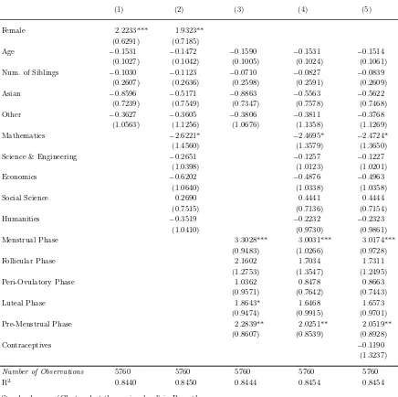
Specification (1) in Table 2 and specification (6) in Table 3 show that there are substantial gender differences, both in terms of bids and total profits.
Observation 1 (Gender) Females bid significantly higher than men. Females’ profits are significantly lower than males.’
Specification (2) in Table 2 and specification (7) in Table 3 reveal that this observation is robust to controlling for educational background. This result is consistent with Chen, Katuˇsˇc´ak and Ozdenoren (2005, 2009).
Specifications (3)-(4) and (8)-(9) include dummies for the menstrual phases. In Table 2 and Table 3 we follow the same definition of the menstrual phases as in Chen, Katuˇsˇc´ak and Ozdenoren (2005, 2009) assuming that all women follow a menstrual cycle standardized to 28 days. We distinguish the menstrual phase (days 1 to 5), the follicular phase (days 6 to 13), the peri-ovulatory phase (days 14 to 15), the luteal phase (days 16 to 23), and the premenstrual phase (days 24 to 28).
Observation 2 (Menstrual Cycle) Females bid significantly higher than men during their menstrual or premenstrual phase. Similarly, females’ profits are significantly lower than males’ profits during their menstrual or premenstrual phase. There is no significant difference in bidding and profits between men and women in the follicular, peri-ovulatory or luteal phase.
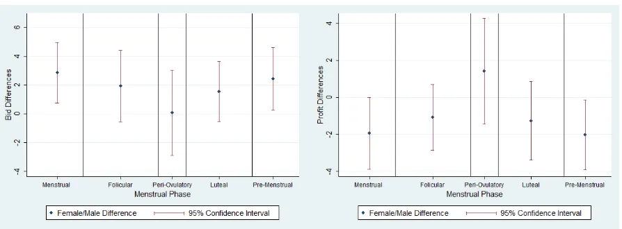
Table 2: Estimated Effects on Bids using 28 Days Standardized Menstrual Cycles
(1) (2) (3) (4) (5)
Female 2.2233*** 1.9323** (0.6291) (0.7185)
Age −0.1531 −0.1472 −0.1590 −0.1531 −0.1514 (0.1027) (0.1042) (0.1005) (0.1024) (0.1061) Num. of Siblings −0.1030 −0.1123 −0.0710 −0.0827 −0.0839
(0.2607) (0.2636) (0.2598) (0.2591) (0.2609) Asian −0.8596 −0.5171 −0.8863 −0.5563 −0.5622
(0.7239) (0.7549) (0.7347) (0.7578) (0.7468) Other −0.3627 −0.3605 −0.3806 −0.3811 −0.3768
(1.0563) (1.1256) (1.0676) (1.1358) (1.1269) Mathematics −2.6221* −2.4695* −2.4724* (1.4560) (1.3579) (1.3650) Science & Engineering −0.2651 −0.1257 −0.1227
(1.0398) (1.0123) (1.0201)
Economics −0.6202 −0.4876 −0.4963
(1.0640) (1.0338) (1.0358)
Social Science 0.2690 0.4441 0.4444
(0.7515) (0.7136) (0.7154)
Humanities −0.3519 −0.2232 −0.2323
(1.0410) (0.9730) (0.9861) Menstrual Phase 3.3028*** 3.0031*** 3.0174***
(0.9483) (1.0266) (0.9728)
Follicular Phase 2.1602 1.7034 1.7311
(1.2753) (1.3547) (1.2495) Peri-Ovulatory Phase 1.0362 0.8478 0.8663
(0.9571) (0.7642) (0.7443)
Luteal Phase 1.8643* 1.6468 1.6573
(0.9474) (0.9915) (0.9701) Pre-Menstrual Phase 2.2839** 2.0251** 2.0519**
(0.8607) (0.8539) (0.8928)
Contraceptives −0.1190
(1.3237)
Number of Observations 5760 5760 5760 5760 5760
R2 0.8440 0.8450 0.8444 0.8454 0.8454
Standard errors (Clustered at the session level) in Parentheses Significance levels: *10%; ** 5%; *** 1%
3.1
Robustness to Menstrual Phases Specifications
One major implicit assumption behind the analysis in our specifications reported in Table 2 and 3 is that all women have a menstrual cycle duration of 28 days. Yet, due to imperfect recall and the intrapersonal variability of the menstrual cycle, retrospective self reports may be an inaccurate measure of the menstrual cycle and the underlying circulating hormone levels. How robust are our results to slight changes in the definitions of the menstrual phases?
Table 3: Estimated Effects on Profits using 28 Days Standardized Menstrual Cycles
(6) (7) (8) (9) (10)
Female −3.3360*** −2.8636** (1.0160) (1.1207)
Age 0.3402 0.3328 0.3632* 0.3525 0.3364 (0.2129) (0.2092) (0.2112) (0.2059) (0.2086) Num. of Siblings −0.1767 −0.1963 −0.2874 −0.3015 −0.2892
(0.3309) (0.3613) (0.3298) (0.3509) (0.3607) Asian 0.8658 0.4141 0.9270 0.4947 0.5477
(1.0528) (1.1743) (1.1005) (1.2179) (1.1872) Other −0.0918 −0.1971 0.0072 −0.0808 −0.1283
(1.4933) (1.6350) (1.5106) (1.6545) (1.6309)
Mathematics 3.3259** 2.9779* 3.0090*
(1.5936) (1.5543) (1.5648) Science & Engineering 1.6149 1.4088 1.3803
(1.4470) (1.4336) (1.4457)
Economics 2.3075 2.0786 2.1537
(1.3862) (1.2669) (1.2967) Social Science 0.3362 −0.0185 −0.0326
(1.1729) (1.1791) (1.1912)
Humanities −0.4838 −0.7067 −0.6215
(1.4982) (1.6225) (1.5943) Menstrual Phase −5.8281*** −5.1962*** −5.3213***
(1.5341) (1.5372) (1.4382) Follicular Phase −2.6258* −2.0126 −2.2835* (1.4635) (1.5424) (1.2192) Peri-Ovulatory Phase 0.2840 0.6216 0.4524
(1.6713) (1.8613) (1.7349) Luteal Phase −2.9394* −2.5019 −2.5960
(1.4762) (1.5789) (1.5308) Pre-Menstrual Phase −3.5938** −3.3403** −3.5781**
(1.4646) (1.5006) (1.4770)
Contraceptives 1.0625
(2.0361)
Number of Observations 192 192 192 192 192
R2 0.2670 0.2929 0.2900 0.3142 0.3153
Standard errors (Clustered at the session level) in Parentheses Significance levels: *10%; ** 5%; *** 1%
cycle. We find substantial variation in cycle length (see Table 1); thus it appears to be relevant for the measurement of menstrual phases. The collected information can be used to construct more individualized menstrual cycles. Individualized phases are constructed in two ways: uniformly adjusted phases and follicular adjusted phases.
Uniformly Adjusted Phases: We uniformly adjust the phases by the individual length of the menstrual cycle. Let
xi :=
Subjecti′s number of days since the first day of the last menstruation period
We define the female subjecti to be in the
1. Uniformly Adjusted Menstrual Phase if and only if xi ≤ 528.5,
2. Uniformly Adjusted Follicular Phase if and only if 5.5
28 < xi ≤ 1328.5,
3. Uniformly Adjusted Peri-ovulatory Phase if and only if 13.5
28 < xi ≤ 16.5
28 ,
4. Uniformly Adjusted Luteal Phase if and only if 16.5
28 < xi ≤ 2328.5,
[image:11.612.146.466.264.668.2]5. Uniformly Adjusted Premenstrual Phase if and only if 23.5 28 < xi.
Table 4: Estimated Effects on Bids using Uniformly Adjusted Phases
(11) (12) (13)
Age −0.1566 −0.1480 −0.1454 (0.0999) (0.1010) (0.1056) Num. of Siblings −0.0753 −0.0915 −0.0931
(0.2639) (0.2637) (0.2650) Asian −0.8666 −0.5558 −0.5660
(0.7224) (0.7547) (0.7406) Other −0.3645 −0.4105 −0.4046
(1.0874) (1.1569) (1.1483) Mathematics −2.3313* −2.3369* (1.3500) (1.3563) Science & Engineering 0.0318 0.0355
(0.9886) (0.9956)
Economics −0.4889 −0.5049
(1.0006) (1.0047) Social Science 0.5765 0.5763
(0.7066) (0.7079) Humanities −0.1175 −0.1359
(0.9173) (0.9321) Uni. Adj. Menstrual Phase 3.1530*** 2.8334** 2.8555***
(0.9640) (1.0572) (1.0100) Uni. Adj. Follicular Phase 2.3721* 1.8960 1.9367
(1.1956) (1.3045) (1.2067) Uni. Adj. Peri-ovular Phase 0.3302 0.0405 0.0687
(1.4441) (1.4544) (1.4281) Uni. Adj. Luteal Phase 1.7971* 1.5271 1.5483
(1.0156) (1.0437) (1.0085) Uni. Adj. Premenstrual Phase 2.5404** 2.3784** 2.4190**
(1.0541) (0.9875) (1.0462)
Contraceptives −0.1893
(1.3291)
Number of Observations 5760 5760 5760
R2 0.8445 0.8456 0.8456
Table 5: Estimated Effects on Profits using Uniformly Adjusted Phases
(14) (15) (16)
Age 0.3582* 0.3421 0.3247
(0.2060) (0.1997) (0.2022) Num. of Siblings −0.2468 −0.2467 −0.2355
(0.3353) (0.3508) (0.3612)
Asian 0.8531 0.4546 0.5171
(1.0981) (1.2359) (1.1945) Other −0.1909 −0.1920 −0.2359
(1.5570) (1.7214) (1.6937)
Mathematics 2.8789* 2.9164*
(1.6200) (1.6283) Science & Engineering 1.1110 1.0866
(1.4535) (1.4615)
Economics 2.1081* 2.2025*
(1.2041) (1.2432) Social Science −0.1805 −0.1933
(1.2126) (1.2235)
Humanities −0.7881 −0.6736
(1.6497) (1.6076) Uni. Adj. Menstrual Phase −5.5814*** −4.8755*** −5.0065***
(1.5560) (1.5971) (1.5014) Uni. Adj. Follicular Phase −2.8915* −2.2279 −2.4939* (1.4352) (1.5541) (1.2655) Uni. Adj. Peri-ovular Phase 0.3509 0.9325 0.7663
(2.2147) (2.2017) (2.0176) Uni. Adj. Luteal Phase −2.9071 −2.4278 −2.5516
(1.7373) (1.8070) (1.7662) Uni. Adj. Premenstrual Phase −3.6197** −3.5156** −3.7633**
(1.6281) (1.5876) (1.5526)
Contraceptives 1.1359
(1.9891)
Number of Observations 192 192 192
R2 0.2872 0.3125 0.3138
Standard errors (Clustered at the session level) in Parentheses Significance levels: *10%; ** 5%; *** 1%
Follicular Adjusted Phases: Hampson and Young (2008) write “The length of the luteal phase is relatively fixed at 13 to 15 days. Therefore, most of the variation in cycle length from women to women is attributable to differences in the length of the follicular phase.” Thus, we consider adjusting the length of the follicular phase only. We start by redefine recursively the last three phases starting with the last phase. Letyi be subject
i’s the number of days since the first day of the last menstrual cycle, and di the average
duration of i’s menstrual cycles. Female subjecti is in the
1. Follicular Adjusted Premenstrual Phase if and only if yi > di−5,
Table 6: Estimated Effects on Bids using Follicular Adjusted Phases
(17) (18) (19)
Age −0.1591 −0.1477 −0.1455 (0.1014) (0.1017) (0.1062) Num. of Siblings −0.0562 −0.0736 −0.0748
(0.2712) (0.2734) (0.2744) Asian −0.9228 −0.6122 −0.6206
(0.6915) (0.7202) (0.7096) Other −0.4274 −0.5091 −0.5034
(1.0790) (1.1539) (1.1469) Mathematics −2.3407* −2.3459* (1.3348) (1.3426) Science & Engineering 0.0526 0.0562
(0.9803) (0.9880)
Economics −0.6635 −0.6774
(1.0126) (1.0209)
Social Science 0.6059 0.6058
(0.6830) (0.6846)
Humanities −0.2099 −0.2260
(0.8934) (0.9073) Fol. Adj. Menstrual Phase 3.3097*** 2.9659*** 2.9850***
(0.9442) (1.0235) (0.9689) Fol. Adj. Follicular Phase 1.5095 1.0032 1.0340
(1.1598) (1.2275) (1.1397) Fol. Adj. Peri-ovular Phase −0.0952 −0.4058 −0.3735
(1.7329) (1.6348) (1.6192) Fol. Adj. Luteal Phase 1.8141* 1.4694 1.4862
(1.0146) (1.0478) (1.0134) Fol. Adj. Premenstrual Phase 3.1173*** 2.9915*** 3.0273**
(1.0721) (1.0272) (1.0958)
Contraceptives −0.1605
(1.2824)
Number of Observations 5760 5760 5760
R2 0.8449 0.8460 0.8460
Standard errors (Clustered at the session level) in Parentheses Significance levels: *10%; ** 5%; *** 1%
Follicular Adjusted Premenstrual Phase,
3. Follicular Adjusted Peri-ovulatory Phase if and only if yi > di−16 and i is not
in the Follicular Adjusted Premenstrual Phase or the Follicular Adjusted Luteal Phase.
Next, female subjecti is in the
4. Follicular Adjusted Menstrual Phase if and only if i is in the Menstrual Phase.
Table 7: Estimated Effects on Profits using Follicular Adjusted Phases
(20) (21) (22)
Age 0.3616* 0.3410 0.3235
(0.2103) (0.2021) (0.2051) Num. of Siblings −0.2792 −0.2812 −0.2713
(0.3554) (0.3707) (0.3786)
Asian 0.9749 0.5852 0.6450
(1.0654) (1.1916) (1.1541)
Other 0.0418 0.1076 0.0582
(1.5270) (1.6954) (1.6712)
Mathematics 2.6985 2.7396
(1.6369) (1.6499) Science & Engineering 1.0215 0.9948
(1.4283) (1.4357)
Economics 2.3182* 2.4139*
(1.2119) (1.2545) Social Science −0.3243 −0.3373
(1.1909) (1.2020)
Humanities −0.8351 −0.7173
(1.6878) (1.6361) Fol. Adj. Menstrual Phase −5.8237*** −5.1139*** −5.2459***
(1.5290) (1.5289) (1.4343) Fol. Adj. Follicular Phase −2.1249 −1.4701 −1.7057
(1.4280) (1.5311) (1.2443) Fol. Adj. Peri-ovular Phase 1.3448 2.1689 1.9321
(2.5033) (2.2649) (2.1181) Fol. Adj. Luteal Phase −2.5364 −1.9356 −2.0473
(1.6774) (1.7620) (1.7153) Fol. Adj. Premenstrual Phase −4.5599** −4.5286** −4.7830***
(1.6871) (1.6715) (1.6687)
Contraceptives 1.1245
(1.9993)
Number of Observations 192 192 192
R2 0.2978 0.3264 0.3277
Standard errors (Clustered at the session level) in Parentheses Significance levels: *10%; ** 5%; *** 1%
5. Follicular Adjusted Follicular Phase if and only if iis not in the Follicular Adjusted Menstrual Phase, Follicular Adjusted Peri-ovulatory Phase, Follicular Adjusted Luteal Phase or Follicular Adjusted Premenstrual Phase.
The results remain robust when using uniformly or follicular adjusted phases as controls. The results in Tables 4 and 6 (bids) and Tables 5 and 7 (profits) are analogous to specifications (3) to (5) in Table 2 and specifications (8) to (10) in Table 3 except that we replaced the 28 day standardized phases by uniformly adjusted phases and follicular adjusted phases respectively.
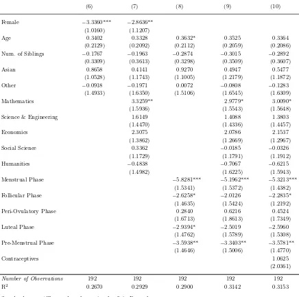
Figure 2: Men-Women Differences of Bids and Profits
3.2
Hormonal Contraceptives and PMS
We also collected information on hormonal contraceptives that may influence hormones and hence behavior along the menstrual cycle. All hormonal contraceptives we encountered in our sample contain progesterone, and some contain only progesterone. Progesterone may have a sedating effect by acting as allosteric modulator of neurotransmitter receptors such as GABA-A.4 Hence, one would expect that progesterone should reduce risk taking,
and thus increase bids on average along the entire cycle except during menstruation. On the other hand, Alexander et al. (1990) report that users of oral contraceptives exhibit higher blood plasma concentrations of testosterone that is thought to be positively associated with aggression although no consistent correlation has been reported for women (Dabbs and Hargrove, 1997). This may suggest higher risk taking by women on hormonal contraceptives. Specifications (5), (10), (13), (16), (19), and (22) reveal that our results remain robust when controlling for hormonal methods of birth control. Hormonal methods of birth control do not have a significant effect on bids. Profits in the follicular phases are significantly lower when controlling for hormonal contraceptives. Yet, we like to point out that only a relatively small number of women (15% of all women in our sample) in our study reported using hormonal contraceptives.
We also collected information on symptoms of pre-menstrual syndrome (PMS). Similar to Chen, Katuˇsˇc´ak and Ozdenoren (2005, 2009), we do not find a significant effect of mild PMS. However, only one subject in our sample reported suffering from severe PMS, thus we cannot draw any inference in this category.
4
3.3
Correlation between Fertility and Competitive Bidding
[image:16.612.120.484.308.530.2]Our finding of significant male/female bid differences during females’ menstrual or pre-menstrual phase and no significant differences in the follicular, peri-ovulatory or luteal phase does not necessarily imply that women in the menstrual or premenstrual phase bid significantly higher than women in the follicular, peri-ovulatory or luteal phase. Table 8 reports the p-values of bidding and profit differences between women in different phases of their menstrual cycle. The results are calculated from specifications (13) and (16) respectively taking into account the uniformly adjusted phases. (Qualitatively similar results obtain using 28-days standardized or follicular adjusted phases.) Only bidding and profits of women in the peri-ovulatory phase are significantly different from the menstrual phase. The peri-ovulatory phase corresponds roughly to the fertile window of the menstrual cycle.
Table 8: p-values of Differences between Women Across the Menstrual Cycle
Bids Follicular Phase Peri-Ovulatory Phase Luteal Phase Premenstrual Phase
Menstruation 0.5270 0.0873* 0.2459 0.7447 Follicular Phase 0.2872 0.7429 0.7692 Peri-Ovulatory Phase 0.3195 0.1945
Luteal Phase 0.5144
Profits Follicular Phase Peri-Ovulatory Phase Luteal Phase Premenstrual Phase
Menstruation 0.1530 0.0144** 0.1984 0.5074 Follicular Phase 0.1496 0.9716 0.5583 Peri-Ovulatory Phase 0.2205 0.1228
Luteal Phase 0.5638
Significance levels: *10%; ** 5%
Observation 3 Females in the fertile phase of the menstrual cycle bid significantly lower than females in other phases of their menstrual cycle. Females in the fertile phase of the menstrual cycle earn significantly more than females in other phases of their menstrual cycle.
with regular and irregular cycles. In that study daily calendars of menstrual information and intercourse were kept and daily urinary hormone assays were collected. Moreover, information about the regularity of menstrual cycles were collected by a questionnaire. We define an irregular cycle to be if a subject reported that her last menstruation is farther away than her typical duration of the menstrual cycle, or if her last menstruation occurred more than 40 days ago, or if her typical duration of her menstrual cycle exceeds 40 days. Otherwise, we assume she has a regular cycle.5
Figure 3: Probability of Conception (Wilcox et al., 2001)
Table 9 and 10 shows regressions on bids and total profits respectively. Bids are lower the higher the probability of conception on a 10% significance level. Total profits are higher the higher the probability of conception on a 5% significance level. The magnitudes are substantial. A 1% increase in the probability of conception translates into US$ 0.50 higher total profit. These findings are robust to the inclusion of controls for majors and hormonal contraceptives.
3.4
Further Observations
Chen, Katuˇsˇc´ak and Ozdenoren (2005) report that subjects with siblings bid significantly lower than those without. They suggest that subjects with siblings may have developed a preference for competitive situations and consequently behave more risk taking. Chen, Katuˇsˇc´ak and Ozdenoren (2009) do not report results on the number of siblings, but the
5
Table 9: Correlation between Bids and the Prob. of Conception
(23) (24) (25)
Female 2.8678*** 2.5753*** 2.5848*** (0.6745) (0.7481) (0.7220) Age −0.1526 −0.1465 −0.1457
(0.0997) (0.1018) (0.1054) Num. of Siblings −0.0829 −0.0905 −0.0910
(0.2609) (0.2628) (0.2639) Asian −0.8732 −0.5301 −0.5332
(0.7331) (0.7598) (0.7501) Other −0.2419 −0.2420 −0.2392
(1.0786) (1.1403) (1.1337) Mathematics −2.5845* −2.5876* (1.4284) (1.4395) Science & Engineering −0.2514 −0.2509
(1.0344) (1.0364) Economics −0.5833 −0.5892
(1.0549) (1.0570) Social Science 0.3265 0.3254
(0.7439) (0.7401) Humanities −0.3939 −0.4017
(1.0638) (1.0768) Prob. of Conception −25.6916* −25.4997* −25.4661* (14.0541) (13.0833) (12.9778)
Contraceptives −0.0657
(1.2080)
Number of Observations 5760 5760 5760
R2 0.8445 0.8455 0.8455
Standard errors (Clustered at the session level) in Parentheses Significance levels: *10%; ** 5%; *** 1%
authors kindly provided us the results (private communication). Overall, they also find that subjects with siblings bid significantly lower than those without. Yet, if only the new data are considered (see subsection 5.1 for a discussion of the data sets), then there is no significant effect. We do not find that the number of siblings significantly affect bidding or profits. This is the case whether we control for the number of siblings linearly or using an indicator for whether participants have siblings or not.
Table 10: Correlation between Profits and the Prob. of Conception
(26) (27) (28)
Female −4.6555*** −4.1482*** −4.2868*** (1.1350) (1.1963) (1.1160) Age 0.3445 0.3367 0.3233
(0.2066) (0.2036) (0.2071) Num. of Siblings −0.2232 −0.2472 −0.2397
(0.3321) (0.3593) (0.3675) Asian 0.9009 0.4487 0.4944
(1.0923) (1.2024) (1.1640) Other −0.3059 −0.4100 −0.4586
(1.5252) (1.6591) (1.6407) Mathematics 3.2463* 3.2973* (1.5842) (1.6080) Science & Engineering 1.6359 1.6312
(1.4337) (1.4458)
Economics 2.2491* 2.3374*
(1.2904) (1.3255) Social Science 0.2664 0.2744
(1.1484) (1.1465) Humanities −0.4022 −0.2804
(1.4004) (1.3641) Prob. of Conception 52.9892** 51.1310** 50.5109**
(20.9389) (20.5414) (20.1024)
Contraceptives 0.9647
(1.9444)
Number of Observations 192 192 192
R2 0.2854 0.3100 0.3109
Standard errors (Clustered at the session level) in Parentheses Significance levels: *10%; ** 5%; *** 1%
4
An Evolutionary Hypothesis
Our results show roughly that women bid more riskily in times of high fertility. Their bids do not significantly differ from men in their fertile phase, but women bid significantly higher than men in their infertile phases. This suggests an evolutionary explanation: risky bidding may just be correlated with general risky behavior of women during their fertile period. Risky behavior may lead to a higher probability of conception, genetic diversity and higher quality offsprings through extrapair mating. This may be especially successful in monogamous societies where some females must end up with substandard males. Thus females with risky behavior near ovulation may have a higher reproductive success. On one hand, extrapair mating is risky because it is punished severely in most societies6 and
may lead to a loss of the long term mating partner who supports child rearing. There is some evidence for greater mate guarding near ovulation (see Gangestad, Thorndill, and
6
Garver, 2002, and Haselton and Gangestad, 2006), which may be a long-term male mate’s best response to riskier behavior of the female during her fertile window and may in turn requires more risky behavior of females to escape the guard. On the other hand, men of higher genetic quality tend to have poorer parental qualities (Gangestad and Simpson, 2000). To maximize the quality of the genetic endowment, a women should have the highest propensity to extrapair mating during their fertile period. Bressan and Stranieri (2008) show that partnered women favor single men with more masculine features during their fertile phase, while they prefer attached men during their low-fertility phase.7 Wilcox
et al. (2004) show that the frequency of intercourse increases during the fertile period.8
Our evolutionary hypothesis could be questioned in various ways. For instance, why should women be more risk averse than men in the first place? An answer may be given based on the “sperm-is-cheap-eggs-are-costly” hypothesis (Bateman, 1948, Trivers, 1972). In principle, a male has abundant sperm till old age while the number of fertile windows in a woman’s life is relatively small (about 400). Since the total number of offsprings produced by all males must equal the number of offsprings of all females, the females become the limiting resource. Competition for female mating partners among men is similar to a winner-take-all contest in which the most successful men can mate with a larger number of women. For winner-take-all games, Dekel and Scotchmer (1999) show conditions under which risk taking behavior emerges in an evolutionary process. An alternative answer may be based on a model by Robson (1996). He considers a population composed of an equal number of males and females, in which females are identical and males are differentiated by wealth. A variable number of females may choose a male, and offspring is produced by a concave production function featuring wealth and females as input. Individuals can select fair bets. For any nontrivial distribution of wealth levels, equilibrium involves some males gambling and women behaving strictly risk averse (see Robson, 1996, for details).
At this point, it may be appropriate to discuss any seemingly contrary evidence to our evolutionary hypothesis. Indeed, at a first glance, our main result that women behave more risk taking during their fertile phase of their cycle seems to contrast a study by Br¨oder and Hohmann (2003). In their study, a group of 23 women rated daily activities according by their “riskiness.” 51 women reported their daily activities on four occasions. A menstrual calendar was used to collect menstrual information. The author find that women near ovulation report less “risky” daily activities than away from ovulation. No such effect was found for women using oral contraceptives (about half of their sample). The authors hypothesis is that women near ovulation take less chances of being raped. Yet, most of the “risky” activities they describe may be interpreted as risks in the sexual “loss” domain rather than the sexual “gain” domain. To reconcile their finding with our result, we may distinguish analogously to Kahneman and Tversky’s (1979) fundamental
7
For related evidence, see Gangestad, Thornhill, and Garver-Apgar (2006), Penton-Voak et al. (1999), and Penton-Voak and Perrett (2000).
8
distinction of losses and gains for choice under uncertainty in prospect theory between a sexual loss domain and a sexual gain domain with respect to parental investment (both in terms of genetic qualities and resources to raise offsprings). Rapists do not provide resources to raise offsprings and may have lower genetic qualities than a mating partner who competed successfully against other males by showing his qualities in courtship and has been actively selected for that by the women. So from an evolutionary point of view, one may speculate that women may be adapted to behave in their fertile window more risk averse in the loss domain but more risk taking in the gain domain as compared to menstruation and the premenstrual phase. A test of this hypothesis is left for further research.
5
Chen, Katuˇ
sˇ
c´
ak and Ozdenoren (2005, 2009)
We designed our experiment with full knowledge of Chen, Katuˇsˇc´ak and Ozdenoren (2005) but before the circulation of Chen, Katuˇsˇc´ak and Ozdenoren (2009). Since the results of Chen, Katuˇsˇc´ak and Ozdenoren (2009) differ from Chen, Katuˇsˇc´ak and Ozdenoren (2005), we discuss in this section differences of our experiment to both Chen, Katuˇsˇc´ak and Ozdenoren (2005) and Chen, Katuˇsˇc´ak and Ozdenoren (2009). Even though Chen, Katuˇsˇc´ak and Ozdenoren (2009) is a substantial revision of Chen, Katuˇsˇc´ak and Ozdenoren (2005), we find the earlier version of the paper still relevant since its conclusions have been quoted in the recent literature. For instance, Apicella et al. (2008) write “... Chen, Katuˇsˇc´ak, and Ozdenoren (2005) find that women in the menstrual phase of their cycle, when estrogen and progesterone are low, are more risk-taking during bid in a first price auction ..., whereas during other phases of the menstrual cycle, they are more risk averse.” This summary is inconsistent with the revision, Chen, Katuˇsˇc´ak and Ozdenoren (2009), in which the authors conclude that women bid higher than men in all phases of their menstrual cycle. Moreover, the authors conclude that higher bidding in the follicular phase and lower bidding in the luteal phase is driven entirely by oral hormonal contraceptives.
We used the same auction program as Chen, Katuˇsˇc´ak and Ozdenoren (2005, 2009). We are extremely grateful to Yan Chen for providing us the program. This program runs on z-tree (Fischbacher, 2007).
5.1
Differences in Designs
The differences between our treatment and the treatments of Chen, Katuˇsˇc´ak and Ozde-noren (2005, 2009) are follows:
Our focus on one treatment
prices, (4) sealed bid first price auction with unknown distribution and auctioneer/reserve prices, (5) sealed bid second price auction with known distribution, (6) sealed bid second price auction with unknown distribution, (7) sealed bid second price auction with known distribution and auctioneer/reserve prices, and (8) sealed bid second price auction with unknown distribution and auctioneer/reserve prices. They report results on the first price auctions pooling data on treatments (1) to (4). To reduce potential confounds, Chen, Katuˇsˇc´ak and Ozdenoren (2009) do not include anymore treatments with auctioneers, i.e. (3) - (4) and (7) - (8), but include an additional treatment on sealed bid first price auc-tions with known distribution (without auctioneer/reserve prices) and a Hold and Laury (2002) lottery choice task. So it is important to note that data in Chen, Katuˇsˇc´ak and Ozdenoren (2005) overlap with Chen, Katuˇsˇc´ak and Ozdenoren (2009) but former contain also data not contained in the latter and vice versa. This raises the question whether differing conclusions in Chen, Katuˇsˇc´ak and Ozdenoren (2009) and Chen, Katuˇsˇc´ak and Ozdenoren (2005) are due to adding some new data or due to excluding some of the old data. Although Chen, Katuˇsˇc´ak and Ozdenoren (2009) do not discuss this issue, we are very grateful to them for having received additional information (private communication) that we discuss below.
Our treatment is identical to their treatment (1). We focused on treatment (1) only in order to eliminate as many confounding factors as possible. We believe that treatments with unknown distributions were included by Chen, Katuˇsˇc´ak and Ozdenoren (2005) in order to study ambiguity in auctions, which was subsequently reported in Chen, Katuˇsˇc´ak and Ozdenoren (2007).
Elicitation of menstruation related information
The measurement of the menstrual cycle relies on selfreports. Selfreports are just a noisy measure of the menstrual cycle but are easy to obtain. Some women may have imperfect recall of when their last menstruation started. Moreover, the length of the menstrual cycle may change due to stress and other environmental factors so that the next onset of menstruation may be difficult to predict correctly. Thus the measurement error may depend crucially on how selfreports are elicited.
Chen, Katuˇsˇc´ak and Ozdenoren (2005) ask “How many days away is your next men-strual cycle?” and construct a prospective measure.9 Chen, Katuˇsˇc´ak and Ozdenoren
(2009) supplement this in the new experimental sessions by “Are you currently menstruat-ing? Yes/No. If yes, how many days have you been menstruatmenstruat-ing? If no, how many days away are you from your next menstrual cycle?” They use this information to construct of what we call a semi-prospective measure of the menstrual cycle. It uses retrospective or current information in case the woman is menstruation. They pool data of both measures and call it the prospective measure.
Chen, Katuˇsˇc´ak and Ozdenoren (2009) also ask for “What date was the first day of your last menstrual period?” They use this information to construct what we call a
9
date-retrospective measure.
We ask our female subjects “How many days ago was the first day of your last menstrual period?”, and use it to construct a retrospective measure. Compared to the prospective and semi-prospective measure, we believe that it is easier for women to remember the onset of their past menstruation than predicting the onset of the next menstruation. Compared to the date-retrospective measure, we believe that it is easier to remember how many days ago was the onset of past menstruation than the exact date. We do not know of any empirical study that analyzes convincingly the measurement error of each measure.10 Such a study would require a random assignment to various measures,
keeping menstrual calendars, and collection of hormone assays.
Chen, Katuˇsˇc´ak and Ozdenoren (2009) improved the measurement of the menstrual cycle by asking female subjects in the new sessions also about the average length of the menstrual cycle and the average number of days of menstruation. This is analogous to our study. Such information is important since menstrual cycles vary substantially across women, and assuming a standardized 28 menstrual cycle for all women may lead to large measurement errors in the construction of the menstrual phases.
Hormonal Contraceptives
Hormonal contraceptives can intervene with the natural length of the menstrual cycle by controlling certain hormones. Moreover, if one assumes that hormones influence the behavior correlated with the menstrual cycle, then it is extremely important to control for hormonal contraceptives. Chen, Katuˇsˇc´ak and Ozdenoren (2009) include for the new sessions a question on whether a woman is on the pill or not, and if yes what is the name of the pill. So this information is available for a subsample of their study. Their Result 3, namely that higher bidding in the follicular phase and lower bidding in the luteal phase is driven by oral contraceptives, is based on 17 women on the pill.
We ask all of our female subjects about hormone-based contraceptives such as birth control pill, IUD, contraceptive patch, vaginal ring, Norplant, IUS, injection etc., and collected information on its name if known.
Demographics
We conducted the experiment at the Social Science and Data Service Lab at UC Davis in Fall 2007. Therefore, the demographics of our subjects are slightly different from Chen, Katuˇsˇc´ak and Ozdenoren (2005, 2009) using their subject pool at the University of Michigan. Table 1 provides the summary statistics of demographic characteristics, educational background and about the menstrual cycle.11 In total, we have 192 subjects
10
Chen, Katuˇsˇc´ak and Ozdenoren (2009), Appendix C, provide a comparsion of their date-retrospective measure on one hand and their prospective measure on the other hand. As they mention, the greater precision of estimates based on the prospective measure may be due to the larger sample size.
11
of which are 94 female. Chen, Katuˇsˇc´ak and Ozdeoren (2009) have 160 subjects in the first price auctions.
Moreover, compared to Chen, Katuˇsˇc´ak and Ozdenoren (2005, 2009) we have a larger share of Asians / Asian Americans (58% versus 33% in Chen, Katuˇsˇc´ak and Ozdenoren, 2005, versus 35% in Chen, Katuˇsˇc´ak and Ozdenoren, 2009) and a lower share of Whites (29% versus 54% in Chen, Katuˇsˇc´ak and Ozdenoren, 2005, versus 48% in Chen, Katuˇsˇc´ak and Ozdenoren, 2009). Chen, Katuˇsˇc´ak and Ozdenoren (2005, 2009) do not report demographic variables for first price and second price auctions separately. Differences in the ethnic composition of the sample may matter. For instance, Harlow et al. (1997) show differences in between-subject standard deviation of cycle length and the odds of having cycles longer than 45 days in African-American and European-American young postmenarcheal women. Moreover, ethnic identity may be strongly correlated with dietary preferences. Jakes et al. (2001) report that dietary intake of soybean protein may increase cycle length. Soybean protein is relatively common in Asian food.
Incentives
Our subjects earned about US$ 18.81 with US$ 5.00 as the minimum and US$ 41.23 as the maximum. Average earnings in Chen, Katuˇsˇc´ak and Ozdenoren (2009) are US$ 13.00 in the first price auctions of the old data set and US$ 12.64 in the new data set. (Together with the lottery earnings, subjects received on average US$ 23.16 in the new data set.)
Subjects’ understanding of the experiment
At the beginning of each session, both Chen, Katuˇsˇc´ak and Ozdenoren (2005, 2009) and we use written instructions and a review questionnaire to test the subjects’ understanding of the instructions (see appendix).
Different from Chen, Katuˇsˇc´ak and Ozdenoren (2005, 2009) we added two practice rounds of bidding to facilitate the understanding of the experiment and allow subjects to get comfortable with the computerized auction format. The profit achieved in those two rounds was not included into the subjects’ payment and this was public knowledge. Our conclusions do not change if we include the two practice rounds into the analysis.
Different from Chen, Katuˇsˇc´ak and Ozdenoren (2005, 2009), we also took the scan of each subject’s right hand after the experiment. The analysis of those data is presented in Pearson and Schipper (2009).
5.2
Differences in Results
estimate if it differs from our point estimate more than 1.96 times our standard error. If we compare our estimates in specification (4) (Table 2) with Chen, Katuˇsˇc´ak and Ozdenoren (2005, Specification (4) in Table 4), then we can reject all their point estimates except for the menstrual and premenstrual phases. In private communication the authors kindly provided us regression results on their new data and their pooled data used in Chen, Katuˇsˇc´ak and Ozdenoren (2009). If we consider the new data only analogous to specification (4), then we can not reject any of their point estimates. However, if we consider the pooled data used in Chen, Katuˇsˇc´ak and Ozdenoren (2009), then we can not reject any of their point estimates except for the follicular phase, which is significantly higher than our estimate.
6
Discussion
In an independent replication study analogous to the path-breaking work by Chen, Katuˇsˇc´ak and Ozdenoren (2005, 2009), we show that on average women bid significantly higher than men during menstruation and the premenstrual phase and that there are no significant differences of bidding between men and women in the other phases of the menstrual cycle. These effects translate into profits significantly lower during the premenstrual and menstrual phases. We conclude that women bid more riskily during their fertile window of the menstrual cycle. We suggest an evolutionary explanation whereby risky behavior during the fertile window increases the probability of conception, the quality of offspring, and genetic variety. Our conclusions differ from that of Chen, Katuˇsˇc´ak and Ozdenoren (2005, 2009). Various differences in the designs may contribute to the differences in conclusions. The differences may be a result of lower measurement error due to a different measure of the menstrual cycle and our focus on one treatment only. The differences may be also a result of our different subject pool with a higher fraction of Asians and a higher number of observations. Selfreported days in the menstrual cycle are just a noisy measure of some hormones that may be involved in influencing behavior especially risk taking.
Our results demonstrate a correlation between biological factors and economic behavior. In particular, higher bidding of women during menstruation and the premenstrual phase points to a number of hormones that peak during the mid-cycle such as estradiol, testos-terone, FH and LSH. This is consistent with our evolutionary hypothesis. For instance, Welling et al. (2007) found a positive association between attraction to masculine faces and women’s levels of salivary testosterone. Further studies are required to disentangle which hormones exactly influence competitive behavior. A follow up experiment directly collecting hormone assays from subjects is left for further research.
which rational agents can exercise control over their actions and decisions, then the partial biological determinism of economic behavior may question free will as the implicit underlying hypothesis of welfare economics. Third, biological factors such as hormones may be manipulated by pharmaceutical products. Thus economic performance may be influenced similar to performance in sports by doping - raising similar ethical issues.
While our findings shed some light on the research question, several issues remain that warrant further study. First, the measurement of the menstrual phases could be further improved by measuring hormone levels directly using urinary hormone assays. Second, so far we just hypothesize on the causal effect of hormones on bidding behavior. The causality could be established by experimentally manipulating hormone levels of subjects. Third, it is not evident that the biological factors we observe influence bidding through risk aversion. For instance, higher bids in first price auctions (but not in second price auctions) may also be due to anticipated regret from losing the auction (Filiz and Ozbay, 2007). To test such an hypothesis, we could to conduct third price auctions `a la Kagel and Levin (1993) with many bidders, which would depart substantially from the two-bidder model of Chen, Katuˇsˇc´ak and Ozdenoren (2005, 2007, 2009). In third price auctions, anticipated loser regret and risk aversion predict effects in opposite directions. Fourth, it is intriguing to explore whether women in the fertile period become more risk averse in the loss domain as conjectured at the end of Section 4. Finally, one should explore whether women during their fertile window generally behave more riskily in other decisions involving gains in accordance to our evolutionary hypothesis.
A
Instructions
Introduction
You are about to participate in a decision process in which an imaginary object will be auctioned off for each group of participants in each of 30 rounds. This is part of a study intended to provide insight into certain features of decision processes. If you follow the instructions carefully and make good decisions you may earn a bit of money. You will be paid in cash at the end of the experiment.
During the experiment, we ask that you please do not talk to each other. If you have a question, please raise your hand and an experimenter will assist you.
You may refuse to participate in this study. You may change your mind about being in the study and quit after the study has started.
Procedure
In each of 30 rounds, you will berandomly matched with one other participant into a group. Each group has two bidders. You will not know the identity of the other participant in your group. Your payoff each round depends ONLY on the decisions made by you and the other participant in your group.
In each of 30 rounds, each bidder’s value for the object will be randomly drawn from 1 of 2 distributions:
– with 25% chance it is randomly drawn from the set of integers between 1 and 50, where each integer is equally likely to be drawn.
– with 75% chance it is randomly drawn from the set of integers between 51 and 100, where each integer is equally likely to be drawn.
For example, if you throw a four-sided die, and it shows up 1, your value will be equally likely to take on an integer value between 1 and 50. If it shows up 2, 3 or 4, your value will be equally likely to take on an integer value between 51 and 100.
Low value distribution: If a bidder’s value is drawn from the low value distribution, then
– with 75% chance it is randomly drawn from the set of integers between 1 and 50, where each integer is equally likely to be drawn.
– with 25% chance it is randomly drawn from the set of integers between 51 and 100, where each integer is equally likely to be drawn.
For example, if you throw a four-sided die, and if it shows up 1, 2 or 3, your value will be equally likely to take on an integer value between 1 and 50. If it shows up 4, your value will be equally likely to take on an integer value between 51 and 100.
Therefore, if your value is drawn from the high value distribution, it can take on any integer value between 1 and 100, but it is three times more likely to take on a higher value, i.e., a value between 51 and 100.
Similarly, if your value is drawn from the low value distribution, it can take on any integer value between 1 and 100, but it is 3 times more likely to take on a lower value, i.e., a value between 1 and 50.
In each of 30 rounds, each bidder’s value will be randomly and independently drawn from the high value distribution with 30% chance, and from the low value distribution with 70% chance. You will not be told which distribution your value is drawn from. The other bidders’ values might be drawn from a distribution different from your own. In any given round, the chance that your value is drawn from either distribution does not affect how other bidders’ values are drawn.
Each round consists of the following stages:
Bidders are informed of their private value, and then each bidder will simultaneously and independently submit a bid, which can be any integer between 1 and 100, inclusive.
The bids are collected in each group and the object is allocated according to the rules of the auction explained in the next section.
Bidders will get the following feedback on their screen: your value, your bid, the winning bid, whether you got the object, and your payoff.
The process continues.
Rules of the Auction and Payoffs
In each round,
• if your bid is greater than the other bid, you get the object and pay your bid:
Your Payoff =Your Value - Your Bid;
• if your bid is less than the other bid, you don’t get the object:
• if your bid is equal to the other bid, the computer will break the tie by flipping a fair coin. Such that:
with 50% chance you get the object and pay your bid:
Your Payoff= Your Value - Your Bid;
with 50% chance you don’t get the object:
Your Payoff = 0.
There will be 30 rounds. There will be 2 practice rounds. From the first round, you will be paid for each decision you make.
Your total payoff is the sum of your payoffs in the 30 “real” rounds. The exchange rate is $1 for 13 points.
We encourage you to earn as much cash as you can. Are there any questions?
Review Questions: Please raise your hand if you have any questions. After 5 minutes we will go through the answers together.
1. Suppose your value is 60 and you bid 62. If you get the object, your payoff =. If you don’t get the object, your payoff =.
2. Suppose your value is 60 and you bid 60. If you get the object, your payoff =. If you don’t get the object, your payoff =.
3. Suppose your value is 60 and you bid 58. If you get the object, your payoff =. If you don’t get the object, your payoff =.
4. In each of 30 rounds, each bidder’s value will be randomly and independently drawn from the high value distribution with % chance.
5. Suppose your value is drawn from the low value distribution. With what % chance is the other bidder’s valuation also drawn from the low distribution?
6. True or False:
C
Questionnaire
POST-EXPERIMENT SURVEY Terminal No.:
We are interested in whether there is a correlation between participants bidding behavior and some socio-psychological factors. The following information will be very helpful for our research. This information will be strictly confidential.
1. What is your gender?
MaleFemale
2. What is your ethnic origin?
White Asian/Asian American African AmericanHispanicNative American Other
3. What is your age?
4. How many siblings do you have?
5. Would you describe your personality as (please choose one)
optimisticpessimisticneither
6. Which of the following emotions did you experience during the experiment?
(You may choose any number of them.) angeranxietyconfusioncontentmentfatigue
happinessirritationmood swingswithdrawal
7. What is your major field of study?
Economics Mathematics Other Social Science English Other Arts/Humanities
Chemistry/Biology/PhysicsOther Natural ScienceEngineering
8. For female participants only:
• How many days ago was the first day of your last menstrual period?
• On average, how many days are there between your menstrual cycles?
<252526272829303132333435>35
• How many days does your menstruation last on average?
23 4 5
• Do you currently use a hormone-based contraceptive (birth control pill, IUD, contraceptive patch [OrthoEvra], vaginal ring [Nuvaring], Norplant, IUS, injection [DepoProvera, Lunelle], etc.)? Yes
No. If yes, what type? I do not remember.
References
[2] Apicella, C.L., Dreber, A., Campbell, B., Gray, P.B., Hoffman, M., and Little, A.C. (2008). Testosterone and financial risk preferences, Evolution and Human Behavior 29, 384-390.
[3] Bateman, A.J. (1948). Inrasexual selection in Drosophila, Heridity 2, 349-368.
[4] Blau, F. and Kahn, L. (2000). Gender differences in pay, Journal of Economic Perspectives 14, 75-99.
[5] Bressan, P. and Stranieri, D. (2000). The best men are (not always) already taken, Psycho-logical Science 19, 145-151.
[6] Br¨oder, A., and Hohmann, N. (2003). Variations in risk taking behavior over the menstrual cycle: An improved replication, Evolution and Human Behavior 24, 391-398.
[7] Cameron, C., Gelbach, J., and Miller, D. (2008). Bootstrap-based improvements for inference with clustered errors, Review of Economics and Statistics 90, 414-427.
[8] Casari, M., Ham, J. and Kagel, J. (2007). Selection bias, demographic effects and ability effects in common value auction experiments, American Economic Review 97, 1278-1304.
[9] Case, A. and Paxson, C. (2008). Stature and status: Height, ability, and labor market outcomes, Journal of Political Economy 116, 499-532.
[10] Cesarini, D., Dawes, C.T., Johannesson, M., Lichtenstein, P., and Wallace, B. (2009). Genetic variation in preferences for giving and risk taking, Quarterly Journal of Economics 124, 809-842.
[11] Chen Y., Katuˇsˇc´ak, P. and Ozdenoren, E. (2009). Why can’t a woman bid more like a man?, mimeo.
[12] Chen, Y., Katuˇsˇc´ak, P. and Ozdenoren, E. (2007). Sealed bid auctions with ambiguity: Theory and experiments, Journal of Economic Theory 136, 513-535.
[13] Chen Y., Katuˇsˇc´ak, P. and Ozdenoren, E. (2005). Why can’t a woman bid more like a man?, mimeo.
[14] Croson, R. and Gneezy, U. (2009). Gender differences in preferences, Journal of Economic Literature 47, 1-27.
[15] Dabbs, J.M. and Hargrove, M.F. (1997). Age, testosterone, and behavior among female prison inmates, Psychosomatic Medicine 59, 477-480.
[16] Dekel, E., and Scotchmer, S. (1999). On the evolution of attitudes towards risk in winner-take-all games, Journal of Economic Theory 87, 125-143.
[17] Dreber, A., Apicella, C. L., Eisenberg, D.T.A., Garcia, J.R., Zamoree, R.S., Lume, J.K., and Campbell, B. (2009). The 7R polymorphism in the dopamine receptorD4 gene (DRD4)
is associated with financial risk taking in men, Evolution and Human Behavior 30, 85-92.
[19] Gangestad, S.W. and Simpson, J. A. (2000). The evolution of human mating: Trade-offs and strategic pluralism, Behavioral and Brain Sciences 23, 573-644.
[20] Gangestad, S.W., Thorndill, R., and Garver-Apgar, C.E. (2006). Adaptations to ovulation, Current Directions in Psychological Research 14, 312-316.
[21] Gangestad, S.W., Thorndill, R., and Garver, C.E. (2002). Changes in women’s sexual interests and their partners’ mate-retention tactics across the menstrual cycle: Evidence for shifting conflicts of interest, Proceedings of the Royal Society of London B, Biological Sciences, 269, 975-982.
[22] Gneezy, U., Niederle, M., and Rustichini, A. (2003). Performance in competitive environ-ments: Gender differences, Quartely Journal of Economics 118, 1049 1074.
[23] Greiner, B. (2004). An online recruitment system for economic experiments, in: Kremer, K., Macho, V. (eds.), Forschung und wissenschaftliches Rechnen 2003. GWDG Bericht 63, G¨ottingen: Ges. fr Wiss. Datenverarbeitung, 79-93.
[24] Ham, J. and Kagel, J. (2006). Gender effects in private value auctions, Economics Letters 92, 375-382.
[25] Hampson, E. and Young, E.A. (2008). Methodological issues in the study of hormone-behavior relations in humans: Understanding and monitoring the menstrual cycle, in: Becker. J.B. et al. (Eds.), Sex differences in the brain. From genes to behavior, Oxford University Press, 63-78.
[26] Haselton, M.G., and Gangstad, S.W. (2006). Conditional expression of women’s desires and men’s mate guarding across the ovulatory cycle, Hormones & Behavior 49, 509-518.
[27] Harlow, S.D., Campbell, B., L., X.H., and Raz, J. (1997). Ethnic differences in the length of menstrual cycle during the postmenarcheal period, American Journal of Epidemiology 146, 572-580.
[28] Holt, C. and Laury, S. (2002). Risk aversion and incentive effects, American Economic Review 92, 1644-1655.
[29] Ichino, A. and Moretti, E. (2008). Biological gender differences, absenteeism and the earning Gap, American Economic Journal: Applied Economics 1, 183-218.
[30] Jakes, R.W., Alexander, L., Duffy, S.W., Leong, J., Chen, L.H., and Lee, W.H. (2001). Dietary intake of soybean protein and menstrual cycle length in pre-menopausal Singapore Chinese women, Public Health Nutrition 4, 191-196.
[31] Kagel, J. and Levin, D. (1993). Independent private value auctions: Bidder behavior in first, second and third price auctions with varying numbers of bidders, Economic Journal 103, 868-879.
[33] Kanazawa, S. and Kovar, J.L. (2004). Why beautiful people are more intelligent, Intelligence 32, 227-243.
[34] Kosfeld, M., Heinrichs, M., Zak, P., Fischbacher, U. and Fehr, E. (2005). Oxytocin increases trust in humans, Nature 435, 673-676.
[35] Krishna, V. (2002). Auction theory, Academic Press.
[36] Filiz, E. and Ozbay, E. (2007). Auctions with anticipated regret: Theory and experiment, American Economic Review 97, 1407-1418.
[37] Pearson, M. and Schipper, B.C. (2009). The Visible Hand: Finger ratio (2D:4D) and competitive behavior, mimeo, The University of California, Davis.
[38] Penton-Voak, I.S. and Perrett D.I. (2000). Female preference for male faces changes cyclically: Further evidence, Evolution and Human Behavior 21, 39-48.
[39] Penton-Voak, I.S., Perrett, D.I., Castles, D.L., Kobayashi, T., Burt, D.M., Murray, L.K., and Minamisawa, R. (1999). Female preferences for male faces changes cyclically, Nature 399, 741-742.
[40] Robson, A. (1996). The evolution of attitudes to risk: Lottery tickets and relative wealth, Games and Economic Behavior 14, 190-207.
[41] Trivers, R. (1972). Parental investment and sexual selection, in: Campbell, B. (ed.), Sexual selection and the descent of man 1871-1971, Chicago: Aldine, 136-179.
[42] Welling, L.L.M., Jones, B.C., DeBruine, L.M., Conway, C.A., Law Smith, M.J., Little, A.C., Feinberg, D.R., Sharp, M.A., and Al-Dujaili, E.A.S. (2007). Raised salivary testosterone in women is associated with increases attraction to masculine faces, Hormones and Behavior 52, 156-161.
[43] Wilcox, A.J., Baird, D. D., Dunson, D.B., McConnaughey, D.R., Kesner, J.S., and Weinberg, C.R. (2004). On the frequency of intercourse around ovulation: Evidence for biological influences, Human Reproduction 19, 1539-1543.
[44] Wilcox, A.J., Dunson, D.B., Weinberg, C.R., Trussel, J., and Baird, D.D. (2001). Likelihood of conception with a single act of intercourse: providing benchmark rates for assessment of post-coital contraceptives, Contraception 63, 211-215.
[45] Zak, P., Kurzban, R. and Matzner, W.T. (2005). Oxytocin is associated with human trustworthiness, Hormones and Behavior 48, 522-527.