Epstein Barr Virus—The Cause of Multiple Sclerosis

http://dx.doi.org/10.4236/jamp.2016.46109

Epstein Barr Virus—The Cause of Multiple

Sclerosis

Katarina Barukčić

1

_{, Ilija Barukčić}

2 1_{Medical University,Sofia, Bulgaria} 2_{Internist, Horandstrasse, Jever, Germany}

Received 9 May 2016; accepted 10 June 2016; published 13 June 2016

Copyright © 2016 by authors and Scientific Research Publishing Inc.

This work is licensed under the Creative Commons Attribution International License (CC BY).

http://creativecommons.org/licenses/by/4.0/

Abstract

Although many studies have found a kind of a relationship between an Epstein-Barr Virus (EBV) and the development of Multiple Sclerosis (MS), a fundamental aspect of this relationship remains uncertain. What is the cause of Multiple Sclerosis (MS)? In this study, we re-analysed the data as published by Wandinger et al. and were able to establish a new insight: without an Epstein-Barr Virus (EBV) infection no development of Multiple Sclerosis (MS). Furthermore, we determined a highly significant causal relationship between Epstein-Barr Virus (EBV) and multiple sclerosis. Altogether, Epstein-Barr Virus (EBV) is the cause of multiple sclerosis (p-value 0.0004251570).

Keywords

Epstein Barr Virus, Multiple Sclerosis

1. Introduction

Multiple Sclerosis (MS) is an unpredictable disease of the central nervous system which disrupts the communi-cation between the brain and other parts of the body. Multiple Sclerosis (MS) can range from relatively benign to somewhat disabling and devastating symptoms. Some of today approved drugs to treat multiple sclerosis in-clude Novantrone (mitoxantrone), teriflunomide, dimethyl fumarate, copolymer I (Copaxone) and forms of beta interferon. Steroids are used to reduce the duration and severity of attacks in some patients suffering from mul-tiple sclerosis. Exercise and physical therapy can help to preserve remaining function. Various aids such as foot braces, canes, and walkers are of use to help patients to remain independent and mobile. Thus far, there is as yet no cure for multiple sclerosis while millions of people are suffering from this many times deadly disease.

and other. Epidemiological, molecular virology and other [1]-[6] studies have been able to establish EBV as a risk factor for the development of Multiple Sclerosis (MS) and provided some evidence that the pathogenesis of multiple sclerosis might involve a response to an EBV infection. Still, the cause of Multiple sclerosis is not identified.

2. Material and Methods

2.1. Definitions

Definition. Bernoulli random variable

Let t= +1,,+N denote an individual Bernoulli trial each with constant success probability p. Let N de-note the number of independent Bernoulli trials (the size of a random sample or of the population).

Definition. The 2 × 2 table

Let At denote a Bernoulli/Binomial distributed random variable. Let p A

( )

t denote the probability of At. Let Bt denote a Bernoulli/Binomial distributed random variable. Let p B

( )

t denote the probability of Bt. Let

( )

t

(

t t

)

p a = p A∩B denote joint distribution of Atand Bt. Let p b

( )

t = p A

(

t∩Bt

)

denote joint distribution of

At and Bt. Let p c

( )

t =p A

(

t∩Bt

)

denote joint distribution of At and Bt. Let p d

( )

t = p A

(

t∩Bt

)

denote joint distribution of A_t and B_t. In general, it is p a

( )

_t +p b

( )

_t +p c

( )

_t +p d

( )

_t =1. Thus far, the relationships before are expressed in the 2 × 2 table (Table 1).

Thus far, let A= ×N p A

( )

_t denote the expectation value. Let A= − = × −N A N

(

1 p A

( )

t

)

denote the ex-pectation value. Let B= ×N p B

( )

_t denote the expectation value. Let B= − = × −N B N

(

1 p B

( )

t

)

denote the expectation value. Let a= ×N p a

( )

_t = ×N p A

(

_t∩B_t

)

denote the expectation value. Let

( )

t

(

t t

)

b= ×N p b = ×N p A ∩B denote the expectation value. Let c= ×N p c

( )

_t = ×N p A

(

_t∩B_t

)

denote the expectation value. Let d = ×N p d

( )

_t = ×N p A

(

_t∩B_t

)

denote the expectation value. Let

( )

( )

( )

( )

(

t t t t

)

N= + + + = ×a b c d N p a +p b +p c +p d denote the size of the sample or the size of the popula-tion. Let A= +a b denote the expectation value of the condition (i.e. a risk factor, the verum population, the exposed group). Let A= +c d denote the expectation value of the non-condition (i.e. the non-exposed group, the control population). Let B= +a c denote the expectation value of the conditioned. Let B= +b d denote the expectation value of the not conditioned. Thus far, the relationships before are expressed in the 2 × 2 table (Table 2).

Definition. Risk ratio or relative risk

Various quantitative techniques are used in Biostatistics to the describe and evaluate relationships among bi-ologic and medical phenomena. Relative risk, defined by Fischer [7] as ψ, is an important [8][9] statistical me-thod used in epidemiologic studies and clinical trials. Let RR(A, B) denote the relative risk. Based on the 2 by 2 table above, the relative risk RR(A, B) is defined as

(

,

)

a a

₍

(

b

)

₎

RR A B

c c d

+ ≡

+ (1)

In epidemiology and statistics, Relative Risk (RR) is the ratio of the probability of an event a occurring under conditions of being exposed to (a + b),the non-exposed to the probability of c occurring under conditions of being exposed to (c + d), the non-exposed group. The Relative Risk (RR) is a widely used measure of associa-tion in epidemiology. A risk ratio RR(A, B) < 1 suggest that an exposure can be considered as being associated with a reduction in risk. A risk ratio RR(A, B) > 1 suggest that an exposure can be considered as being associated with an increase in risk.

Conditions

The following relationships are taken with friendly permission by Ilija Barukčić [10]. Definition. Conditio sine qua non relationship

Let p A

(

_t ←B_t

)

denote [10] the extent to which a condition A is a conditio sine qua non of the conditioned B. The conditio sine qua non relationship is calculated as

(

t t

)

( )

t

( )

t

( )

t

(

( )

t

( )

t

( )

t

)

N a b d A d a B

p A B p a p b p d p a p b p d

N N N N

+ + + +

← ≡ + + = × + + = ≡ ≡ (2)

[image:3.595.141.500.88.411.2]

Table 1. The 2 × 2 table. Probabilities.

Conditioned Bt

Yes No

Condition At

Yes p a

( )

t p b

( )

t p a

( ) ( )

t +p bt =p A

( )

t

No p c

( )

t p d

( )

t p c

( ) ( )

t +p dt =p A

( )

t

( ) ( )

t t

( )

t

p a +p c =p B p b

( ) ( )

t +p dt =p B

( )

t 1

Table 2. The 2 × 2 table. Expectation values.

Conditioned B

Yes No

Condition A

Yes a b a b+ =A

No c d c+ =d A

a c+ =B b+ =d B N

Table 3. Conditio sine qua non.

Conditioned B

Yes No

Condition A

Yes a b a b+ =A

No c = 0 d c+ =d A

a c+ =B b+ =d B N

Definition. Anti conditio sine qua non relationship

Let p A

(

_t− <B_t

)

denote [10] the extent to which a condition A is not a conditio sine qua non of the condi-tioned B. The anti conditio sine qua non relationship is calculated as

(

t t

)

( )

t

(

( )

t

)

1

(

t t

)

N N a b d c

p A B p c p c p A B

N N N

− − −

− < ≡ = ≡ ≡ ≡ − ← (3)

The relationship before is expressed in the following 2 × 2 table (Table 4). Definition. Conditio per quam relationship

Let p A

(

_t →B_t

)

denote [10] the extent to which a condition A is a conditio per quam of the conditioned B. The conditio per quam is calculated as

(

t t

)

( )

t

( )

t

( )

t

(

( )

t

( )

t

( )

t

)

N a c d B d a A

p A B p a p c p d p a p c p d

N N N N

+ + + +

→ ≡ + + = × + + = ≡ ≡ (4)

The relationship before is expressed in the following 2 × 2 table (Table 5). Definition. Anti conditio per quam relationship

Let p A

(

_t> −B_t

)

denote [10] the extent to which a condition A is not a condition per quam of the condi-tioned B. The anti conditio per quam relationship is calculated as

(

t t

)

( )

t

(

( )

t

)

1

(

t t

)

N b N a c d

p A B p b p b p A B

N N N

− − −

> − ≡ = × ≡ ≡ ≡ − → (5)

The relationship before is expressed in the following 2 × 2 table (Table 6). Definition. Conjunction. A and B relationship

[image:4.595.126.519.81.484.2]

Table 4. Anti conditio sine qua non.

Conditioned B

Yes No

Condition A

Yes a = 0 b = 0 a b+ =A

No c d = 0 c+ =d A

a c+ =B b+ =d B N

Table 5. Conditio per quam.

Conditioned B

Yes No

Condition A

Yes a b = 0 a b+ =A

No c d c+ =d A

a c+ =B b+ =d B N

Table 6. Anti conditio per quam.

Conditioned B

Yes No

Condition A

Yes a = 0 b a b+ =A

No c = 0 d = 0 c+ =d A

a c+ =B b+ =d B N

(

t t

)

( )

t

(

( )

t

)

1

(

t t

)

N a N b c d

p A B p a p a p A B

N N N

− − −

∩ ≡ = × = ≡ ≡ − ∩ (6)

The relationship before is expressed in the following 2 × 2 table (Table 7). Definition. Exclusion relationship

Let p A

(

_t∩B_t

)

denote [10] the extent to which a condition Aexcludes the conditioned Band vice versa. The exculsion relationship (the Sheffer stroke) named after Henry M. Sheffer is written as a vertical bar or an up-wards arrow and calculated as

(

t t

)

(

t t

)

(

t t

)

( ) ( ) ( )

t t t

(

( ) ( ) ( )

t t t

)

N

p A B p A B p A B p b p c p d p b p c p d

N

∩ ≡ ≡ ↑ ≡ + + = × + + (7)

or

(

_{t t}

)

(

_{t t}

)

(

_{t t}

)

b c d N a 1

(

_{t t}

)

p A B p A B p A B p A B

N N

+ + −

∩ ≡ ≡ ↑ ≡ ≡ ≡ − ∩ (8)

The relationship before is expressed in the following 2 × 2 table (Table 8). Definition. Disjunction. A or B relationship

Let p A

(

_t∪B_t

)

denote [10] the extent to which the condition A or the conditioned B are given. The inclu-sive disjunction also known as alternation is calculated as

(

t t

)

( )

t

( )

t

( )

t

(

( )

t

( )

t

( )

t

)

1

(

t t

)

N

p A B p a p b p c p a p b p c p A B

N

∪ ≡ + + = × + + ≡ − ∪ (9)

or

(

_{t t}

)

( )

_t

( ) ( )

_{t t} a b c A B a 1

(

_{t t}

)

p A B p A p B p a p A B

N N

+ + + −

The relationship before is expressed in the following 2 × 2 table (Table 9). Definition. Neither A nor B relationship

Let p A

(

_t∪B_t

)

denote [10] the extent to which neither a condition A nor the conditioned B is given. The neitherAnorB relationship was introduced by Charles Sanders Peirce and is known also as Peirce’s arrow too and can be calculated as

(

t t

)

(

t t

)

( )

t

(

( )

t

)

1

(

t t

)

N d N a b c

p A B p A B p d p d p A B

N N N

− − −

∪ ≡ ↓ ≡ = × = ≡ ≡ − ∪ (11)

The relationship before is expressed in the following 2 × 2 table (Table 10). Definition. Equivalence of A and B relationship

Let p A

(

_t <=>B_t

)

denote [10] the extent to which a condition A and the conditioned B are equivalent. The equivalence of A and B is calculated as

(

t t

)

( )

t

( )

t

(

( )

t

( )

t

)

1

(

t t

)

N a d

p A B p a p d p a p d p A B

N N

+

<=> ≡ + = × + = ≡ − >=< (12)

The relationship before is expressed in the following 2 × 2 table (Table 11). Definition. Either A or B relationship

Let p A

(

_t >=<B_t

)

denote [10] the extent to which either the condition Aor the conditioned B is given. The either A or B relationship can be calculated as

(

t t

)

( )

t

( )

t

(

( )

t

( )

t

)

1

(

t t

)

N b c N a d

p A B p b p c p b p c p A B

N N N

+ − −

>=< ≡ + = × + = ≡ ≡ − <=> (13)

[image:5.595.138.504.343.722.2]

The relationship before is expressed in the following 2 × 2 table (Table 12).

Table 7. Conjunction. A and B.

Conditioned B

Yes No

Condition A

Yes a b = 0 a b+ =A

No c = 0 d = 0 c+ =d A

a c+ =B b+ =d B N

Table 8. Exclusion. A excludes B and vice versa.

Conditioned B

Yes No

Condition A

Yes a = 0 b a b+ =A

No c d c+ =d A

a c+ =B b+ =d B N

Table 9. Disjunction. A or B.

Conditioned B

Yes No

Condition A

Yes a b a b+ =A

No c d = 0 c+ =d A

[image:6.595.132.489.81.423.2]

Table 10. Neither A or B relationship.

Conditioned B

Yes No

Condition A

Yes a = 0 b = 0 a b+ =A

No c = 0 d c+ =d A

a c+ =B b+ =d B N

Table 11. Equivalence of A and B.

Conditioned B

Yes No

Condition A

Yes a b = 0 a b+ =A

No c = 0 d c+ =d A

a c+ =B b+ =d B N

Table 12. Either A or B relationship.

Conditioned B

Yes No

Condition A

Yes a = 0 b a b+ =A

No c d = 0 c+ =d A

a c+ =B b+ =d B N

2.2. Material

Patients and Samples

Data and material for this re-analysis were published by Wandinger [11]et al., a study specifically designed to investigate the relation between Multiple Sclerosis (MS) and viral infections. Wandinger et al. examined sera from a large cohort of 163 healthy control subjects (control group) and 108 patients with a diagnosis of clinical-ly definite multiple sclerosis for the presence of human herpes viruses type 1 (HSV-1), HSV-2, cytomegalovirus (CMV) and EBV by the presence of IgG antibodies. In addition, other investigations (i.e. the detection of EBV DNA in all serum samples) were performed. Some of the data of Wandinger et al. data about the prevalence of IgG antibodies in serum samples from Multiple Sclerosis (MS) patients and healthy control subjects are summa-rized in the table shown below (Table 13).

The data of the prevalence of IgG antibodies in serum samples from multiple sclerosis (MS) patients and healthy control subjects are viewed in the following 2 × 2 table (Table 14).

2.3. Methods

2.3.1. The Chi-Squared Distribution

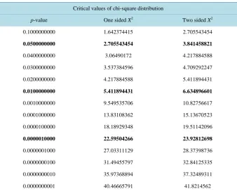
The properties of the chi-squared distribution were first investigated by Karl Pearson [12] in 1900. The chi- squared distribution is a widely used probability distributions in hypothesis testing [14], inferential statistics (Table 15) or in construction of confidence intervals.

In last consequence, the Chi Square with one degree of freedom is nothing but the distribution of a single normal deviate squared.

2.3.2. The Binomial Proportion Confidence Interval

Table 13. Prevalence of IgG antibodies in MS patients and healthy control subjects.

Parameter Multiple Sclerosis (MS) Healthy control subjects

anti-EBNA-1 IgG 108 147

Sample size 108 163

Table 14. EBV and Multiple Sclerosis (MS).

Multiple sclerosis

Yes No

EBV anti-EBNA-1 IgG

Yes 108 147 255

No 0 16 16

[image:7.595.144.483.292.567.2]

108 163 271

Table 15. Chi square distribution for degree of freedom d.f. = 1.

Critical values of chi-square distribution

p-value One sided X2 _{Two sided X}2

0.1000000000 1.642374415 2.705543454

0.0500000000 2.705543454 3.841458821

0.0400000000 3.06490172 4.217884588

0.0300000000 3.537384596 4.709292247

0.0200000000 4.217884588 5.411894431

0.0100000000 5.411894431 6.634896601

0.0010000000 9.549535706 10.82756617

0.0001000000 13.83108362 15.13670523

0.0000100000 18.18929348 19.51142096

0.0000010000 22.59504266 23.92812698

0.0000001000 27.03311129 28.37398736

0.0000000100 31.49455797 32.84125335

0.0000000010 35.97368894 37.32489311

0.0000000001 40.46665791 41.8214562

by a binomial test. For large samples, the binomial distribution is well approximated by convenient Pearson’s chi-squared test. The above relationships are grounded on the assumption, that the number of successes X out of a sample of n observations is equal to X = N. In general, let df1_l denote the degrees of freedom 1 of the f-distribution for the lower confidence bound. Thus far, it is df1_lower = 2

(

N− +X 1

)

. Under conditions where N = X the proportion of success is p X N

(

)

=1, the is then df1_lower= 2. Let df2_lower denote the degrees of freedom 2 of the f-distribution for the lower confidence bound. In particular, we obtain df2_lower= ×2 X . Under conditions where N = X the proportion of success is p X N

(

)

=1 and df2_lower = ×2 N. The exact one-sided lower confidence interval with confidence level 1 − alpha for the proportion of successes p X N

(

)

=1 can be calculated [13] as

( lower lower )

Lower

1 , 2 ,

df df Alpha

N p

N F

=

Example.

Given a sample proportion p and sample size N we can test claims about the population proportion p0.

Differ-ent hypothesis tests and test methods (binomial test, one-sample z-test, the t statistic et cetera) can be used to determine whether a hypothesized population proportion p0 differs significantly from an observed sample

pro-portionp. A hypothesis test requires that a null hypothesis and an alternative hypothesis are mutually exclusive. That is, if a null hypothesis is true, the alternative hypothesis must be false and vice versa. How can we conduct a hypothesis test of a proportion. Especially under conditions, where an observed sample proportion p is equal to 1, the F distribution [13] is of use for these purposes. Thus far, the proportion of successes of our sample above is equal to p X N

(

)

= p

(

271 271

)

=1. Assuming an alpha = 0.05 level of significance the F-value should be calculated as provided above. The F-value for X = N = 271 (Alpha = 0.05) is

1 2, 2 542, 0.05 3.01235141

df df Alpha

F = = = = . The exact one-sided lower confidence bound for the proportion of suc-cesses p X N

(

)

= p

(

271 271

)

=1 follows as

( lower lower )

Lower

1 , 2 ,

271

0.989006512 271 3.01235141

df df Alpha

N p

N F

= = =

+ + (15)

In other words, we assume that the p in the population is greater or equal to 0.989006512. Furthermore, the one- sided lower confidence interval with confidence level 1 − alpha for the proportion of successes p X N

(

)

=1, reflects a significance level of i.e.alpha = 0.05, and can be calculated for N > 50approximately [13] as

Lower

3 1

p

N

≈ − (16)

A 100 × (1 − alpha)% confidence interval consists of all those values p X N

(

)

for which a test of the hy-pothesis p X N

(

)

=1 is not rejected at a significance level of 100 × (alpha)%.

2.3.3. Causal Relationship k

The mathematical formula of the causal relationship k was used to determine the cause-effect relationship be-tween Epstein-Barr Virus (EBV) infections and Multiple Sclerosis (MS). According to Barukčić [14], the causal relationship k is calculated as

(

)

( )

( ) ( )

( )

(

( )

)

( )

(

( )

)

(

) (

)

2 2 , 1 1

t t t

t t

t t t t

p a p A p B N a A B

k A B

A A B B

p A p A p B p B

− × × − ×

≡ ≡

× × ×

× − × × − (17)

The relationship before is expressed in the following 2 × 2 table (Table 16). Pearson’s chi-squared test X²

(

) (

)

(

)

(

(

) (

)

)

(

) (

) (

) (

)

2 N a d b c a d b c

a b c d a c b d

χ ≡ × × − × × × − ×

+ × + × + × + (18)

is used to evaluate how likely it is that the observed causal relationship k arose by chance. The 2 × 2 contingen-cy table is dichotomous while the statistical X2 distribution is continuous. Thus far, Pearson’s chi-square test tends to make results larger than they should be and is biased upwards on this account. This upwards bias of Pearson’s chi-square test can be corrected by using Yates correction.

Scholium.

As a response to Yules association of two attributes Karl Pearson introduced the mean square contingency[15]

into statistics as

Table 16. The causal relationship k.

Effect B

Yes No

Cause A

Yes a b a b+ =A

No c d c+ =d A

(

) (

)

(

)

(

(

) (

)

)

(

) (

) (

) (

)

2 a d b c a d b c

a b c d a c b d

φ ≡ × − × × × − ×

+ × + × + × + (19)

Still, Pearson failed to derive a mathematical formula of the causal relationship k and much more than this. Pearson himself exterminated any kind causation from statistics ultimately. Following Pearson, “We are now in a position, I think, to appreciate the scientific value of the word cause. Scientifically, cause… is meaningless…”

[14]. According to Pearson, the words cause and effect belong strictly to the sphere of sense-impressions. Thus far, “there is… no true cause and effect” [14]. The reader can hardly fail to have been impressed that Pearson himself denies any kind of causality. In the first place, there is no causation at all. “No phenomena are causal”

[14]. Finally, “The wider view of the universe sees all phenomena as correlated, but not causally related” [14]. Consequently, Pearson demands that “… there is association but not causation” [14]. We have now reached some very important conclusions about Pearson’s account for causality. Due to Pearson, there is no causation at all. Thus far, neither Pearson’s correlation coefficient nor his mean square contingency can be regarded as the mathematical formula of the causal relationship k. In particular, Pearson failed to derive and to provide a self-consistent mathematical proof of a mathematical formula of the causal relationship.

2.3.4. Statistical Analysis

Data were analyzed using Microsoft Excel version 14.0.7166.5000 (32-Bit) software (Microsoft GmbH, Munich, Germany). The mathematical formula of the causal relationship k[14] and the chi-square distribution [12] were applied to determine the significance of causal relationship between EBV and multiple sclerosis (MS). A p value of <0.05 was considered significant.

3. Results

3.1. Clinical Characteristics

Wandinger [11] et al. examined 108 MS patients from the Department of Neurology (University of Lübeck School of Medicine). All patients were examined independently by two neurologists and had a diagnosis of clinically definite MS. Kurtzke’s functional systems and Expanded Disability Status Scale (EDSS) were used to grade the physical disability.

3.2. EBV Seropositivity

The viral status was classified by following serologic definitions. Wandinger [11]et al. defined primary EBV infection by positivity of anti-EA-IgG and/or anti-EA-IgM in the absence of anti-EBNA-1 antibodies. A latent or past EBV infection was defined by positivity of anti-EBNA-1 antibodies. A reactivation of a latent EBV in-fection was defined by EBNA-1-IgG-positive individuals by additional positive anti-EA-IgG and anti-EA-IgM or additional high anti-EA-IgM. The marker for latent EBV infection was defined by an EBV nuclear anti-gen type 1 (anti-EBNA-1) immunoglobulin (Ig)G antibodies.

3.3. Epstein Barr Virus (EBV) Is a

Conditio Sine Qua Non

of Multiple Sclerosis (MS)

A hypothesis test is used to distinguish between the null hypothesis and the alternative hypothesis.

Theorem 1.

Null hypothesis: EBV is a conditio sine qua non of multiple sclerosis (MS) (p0≥ p).

Alternative hypothesis: EBV is not a conditio sine qua non of multiple sclerosis (MS) (p0 < p).

Significance level (Alpha) below which the null hypothesis will be rejected: 0.05. Proof by a statistical hypothesis test.

The data of the prevalence of IgG antibodies in serum samples from Multiple Sclerosis (MS) patients and healthy control subjects are viewed in the following 2 × 2 table (Table 17).

The proportion of successes p A

(

_t ←B_t

)

of the condition sine qua non relationship in the sample or the test statistic can be calculated defined before as

(

)

108 147 16 247

1

271 247

t t

a b d A d a B

p A B

N N N

+ + + + + +

The critical value plower is calculated approximately as

Lower

3 3

1 1 0.988929889

247

p

N

≈ − = − = (21)

The critical value plower = 0.989006512 and is less than the proportion of successes p A

(

t ←Bt

)

=1 as ob-tained from the observations (significance level alpha = 0.05).

Conclusio.

We cannot reject the null hypothesis in favor of the alternative hypotheses. The sample data do support the Null hypothesis that Epstein Barr Virus (EBV) is a conditio sine qua non of Multiple Sclerosis (MS).

In other words, without an infection with Epstein Barr Virus (EBV) no development of multiple sclerosis (MS).

Quod erat demonstrandum.

3.4. Epstein Barr Virus (EBV) Is the Cause of Multiple Sclerosis (MS)

Theorem 2.

Conditions. Alpha level = 5%.

The two tailed critical Chi square value (degrees of freedom = 1) for alpha level 5% is 3.841458821. Claims.

Null hypothesis (H0): k = 0 (No causal relationship).

There is no causal relationship between Epstein Barr virus (EBV) and multiple sclerosis (MS). Alternative hypothesis (HA): k ≠ 0 (Causal relationship).

There is a significant causal relationship between Epstein Barr virus (EBV) and multiple sclerosis (MS). Proof by two sided hypothesis test.

Based on the data (Table 18) of Wandinger et al., we compute the causal relationship k(EBV, MS)Obtained (our

test statistic) as

(

)

Obtained

(

2

) (

)

2

271 108 255 108

EBV, MS 0.2038956576.

108 163 255 16

N a A B

k

A A B B

× − × × − ×

≡ = = +

× × × × × × (22)

Following Barukčić, the test statistics obtained is equivalent with a X2 value of

(

)

(

)

(

)

2

2

Obtained Obtained

EBV, MS EBV, MS 271 0.2038956576 11.2664020209.

k k N

χ ≡ × × = × = (23)

A two tailed Chi square of 11.2664020209 is equivalent to a p-value of 0.0004251570.

Table 17. Without EBV no Multiple Sclerosis (MS).

Multiple sclerosis

Yes No

EBV anti-EBNA-1 IgG

Yes 108 147 255

No 0 16 16

108 108 271

Table 18. EBV and Multiple Sclerosis (MS).

Multiple sclerosis

Yes No

EBV anti-EBNA-1 IgG

Yes 108 147 255

No 0 16 16

Conclusio.

The value of the test statistic (k obtained or Chi square calculated) is 11.2664020209 and exceeds the critical Chi square value of 3.841458821. Consequently, we reject the null hypothesis (H0) and accept the alternative

hypothesis (HA).

There is a highly significant causal relationship between Epstein Barr virus (EBV) and multiple sclerosis (k = +0.2038956576, p-value 0.0004251570).

Quod erat demonstrandum.

4. Discussion

Today, the etiology of Multiple Sclerosis (MS) is largely unknown but Multiple Sclerosis (MS) is rare among individuals without serum EBV antibodies. Thus far, there is an accumulating literature for a role of Epstein- Barr Virus (EBV) infections in the pathogenesis of Multiple Sclerosis (MS). Especially, several epidemiological studies suggested an association between infection with Epstein-Barr Virus (EBV) and the occurrence of Mul-tiple Sclerosis (MS) disease. In particular, a recent large prospective epidemiological study showed a relation-ship between an increase of serum antibody titres against EBV before onset of MS. Acherio et al.[16] con-ducted a prospective, nested case-control study of 62,439 women participating in the Nurses’ Health Study to determine whether elevation in serum antibody titers to EBV precede the occurrence of Multiple Sclerosis (MS). Acherio et al. concluded that EBV is associated with the etiology of multiple sclerosis. Recently, Levin et al.

[17] conducted a study among more than 3 million US military personnel and found a relationship between EBV infection and development of MS. Apart from these and other studies aiming at the aetiology of multiple sclero-sis (MS), the cause of Multiple Sclerosclero-sis (MS) has still not been identified.

We conducted a re-analysis of the study of Wandinger [11]et al. to re-investigate the role between EBV in-fection and MS disease. Using some of the data obtained by the study of Wandinger et al., we questioned whether Epstein-Barr Virus (EBV) is the cause or a cause of multiple sclerosis (MS). The study of Wandinger et al. was properly constructed. In accordance with previous studies, Wandinger et al. found an unexpectedly high seropositivity rate in MS patients for EBV compared with control subjects. Wandinger et al. observed an associ-ation of the EBV with MS but failed to detect the true meaning of Epstein-Barr virusin the pathogenesis of mul-tiple sclerosis (MS).

In addition, our study confirms a conditio sine qua non relationship between EBV infection and Multiple Sclerosis (MS). In other words, without an infection with Epstein-Barr Virus (EBV) no development of Multiple Sclerosis (MS) (significance level alpha = 0.05). We observed a highly significant causal relationship between Epstein-Barr Virus (EBV) and multiple sclerosis (k = +0.203895658, p value = 0.000425157). A particular as-pect of our study is the identification of Epstein-Barr Virus (EBV) as the cause of multiple sclerosis. Since without an infection by Epstein-Barr Virus (EBV) no multiple sclerosis develops and due to the fact that there is a highly significant causal relationship between Epstein-Barr Virus (EBV) and multiple sclerosis, we are al-lowed to deduce that Epstein-Barr Virus (EBV) is not only a cause but the cause of Multiple Sclerosis (MS).

5. Conclusion

A particular aspect of our study is the identification of Epstein-Barr Virus (EBV) as the cause of Multiple Scle-rosis (MS). Finally, the cause of multiple scleScle-rosis is identified. Consequently, it is more than necessary to de-velop a low-cost and highly effective vaccine against Epstein-Barr Virus (EBV).

References

[1] Bray, P.F., Bloomer, L.C., Salmon, V.C., Bagley, M.H. and Larsen, P.D. (1983) Epstein-Barr Virus Infection and

An-tibody Synthesis in Patients with Multiple Sclerosis. Archives of Neurology, 40, 406-408. http://dx.doi.org/10.1001/archneur.1983.04050070036006

[2] Sumaya, C.V., Myers, L.W., Ellison, G.W. and Ench, Y. (1985) Increased Prevalence and Titer of Epstein-Barr Virus

Antibodies in Patients with Multiple Sclerosis. Annals of Neurology, 17, 371-377. http://dx.doi.org/10.1002/ana.410170412

[3] Larsen, P.D., Bloomer, L.C. and Bray, P.F. (1985) Epstein-Barr Nuclear Antigen and Viral Capsid Antigen Antibody

Titers in Multiple Sclerosis. Neurology, 35, 435-438. http://dx.doi.org/10.1212/WNL.35.3.435

Neurology, 39, 825-829. http://dx.doi.org/10.1212/WNL.39.6.825

[5] Ascherio, A. and Munch, M. (2000) Epstein-Barr Virus and Multiple Sclerosis. Epidemiology, 11, 220-224. http://dx.doi.org/10.1097/00001648-200003000-00023

[6] Hernan, M.A., Zhang, S.M., Lipworth, L., Olek, M.J. and Ascherio, A. (2001) Multiple Sclerosis and Age at Infection

with Common Viruses. Epidemiology, 12, 301-306. http://dx.doi.org/10.1097/00001648-200105000-00009 [7] Fisher, R.A. (1935) The Logic of Inductive Inference. Journal of the Royal Statistical Society, 98, 39-82.

http://dx.doi.org/10.2307/2342435

[8] Gart, J.G. (1962) Approximate Confidence Limits for the Relative Risk. Journal of the Royal Statistical Society, Series B (Methodological), 24, 454-463.

[9] Gart, J.J. (1962) On the Combination of Relative Risks. Biometrics, 18, 601. http://dx.doi.org/10.2307/2527905 [10] Barukčić, I. (1989) Causality I. A Theory of Energy, Time and Space. 5th Edition, 19th Revision 2011, Lulu,

Morris-ville, 648.

[11] Wandinger, K., Jabs, W., Siekhaus, A., Bubel, S., Trillenberg, P., Wagner, H., Wessel, K., Kirchner, H. and Hennig, H. (2000) Association between Clinical Disease Activity and Epstein-Barr Virus Reactivation in MS. Neurology, 55, 178- 184. http://dx.doi.org/10.1212/WNL.55.2.178

[12] Pearson, K. (1900) On the Criterion That a Given System of Deviations from the Probable in the Case of a Correlated

System of Variables Is Such That It Can Be Reasonably Supposed to Have Arisen from Random Sampling.

Philo-sophical Magazine Series 5, 50, 157-175. http://dx.doi.org/10.1080/14786440009463897

[13] Sachs, L. (1992) Angewandte Statistik: Anwendung statistischer Methoden. Siebte, völlignuebearbeitete Auflage.

Springer, Berlin, 439. http://dx.doi.org/10.1007/978-3-662-05747-6

[14] Barukčić, I. (2016) The Mathematical Formula of the Causal Relationship k. International Journal of Applied Physics and Mathematics, 6, 45-65. http://dx.doi.org/10.17706/ijapm.2016.6.2.45-65

[15] Pearson, K. (1904) Mathematical Contributions to the Theory of Evolution. XIII. On the Theory of Contingency and

Its Relation to Association and Normal Correlation. Dulau and Co., London, 426.

[16] Ascherio, A., Munger, K.L., Lennette, E.T., Spiegelman, D., Hernán, M.A., Olek, M.J., Hankinson, S.E. and Hunter,

D.J. (2001) Epstein-Barr Virus Antibodies and Risk of Multiple Sclerosis: A Prospective Study. Journal of the Ameri-can Medical Association, 286, 3083-3088. http://dx.doi.org/10.1001/jama.286.24.3083

[17] Levin, L.I., Munger, K.L., Rubertone, M.V., Peck, C.A., Lennette, E.T., Spiegelman, D. and Ascherio, A. (2003) Mul-tiple Sclerosis and Epstein-Barr Virus. Journal of the American Medical Association, 289, 1533-1536.