http://dx.doi.org/10.4236/ajcm.2013.34036
Half-Step Continuous Block Method for the Solutions of
Modeled Problems of Ordinary Differential Equations
A. A. James1, A. O. Adesanya2, J. Sunday3, D. G. Yakubu4 1Department of Mathematics, American University of Nigeria, Yola, Nigeria 2Department of Mathematics, Modibbo University of Technology, Yola, Nigeria 3Department of Mathematical Sciences, Adamawa State University, Mubi, Nigeria 4Department of Mathematics, Tafawa Balewa Federal University of Bauchi, Bauch State, Nigeria
Email: [email protected]
Received July 27, 2013; revised August 29, 2013; accepted September 18,2013
Copyright © 2013 A. A. James et al. This is an open access article distributed under the Creative Commons Attribution License,
which permits unrestricted use, distribution, and reproduction in any medium, provided the original work is properly cited.
ABSTRACT
In this paper, we developed a new continuous block method using the approach of collocation of the differential system and interpolation of the power series approximate solution. A constant step length within a half step interval of integra- tion was adopted. We evaluated at grid and off grid points to get a continuous linear multistep method. The continuous linear multistep method is solved for the independent solution to yield a continuous block method which is evaluated at selected points to yield a discrete block method. The basic properties of the block method were investigated and found to be consistent and zero stable hence convergent. The new method was tested on real life problems namely: SIR model, Growth model and Mixture Model. The results were found to compete favorably with the existing methods in terms of accuracy and error bound.
Keywords: Approximate Solution; Interpolation; Collocation; Half Step; Converges; Block Method
1. Introduction
We consider the numerical solution of first order initial value problems of the form:
, ,
0y f x y y x y0 (1)
where f is continuous and satisfies Lipchitz’s condition
that guarantees the uniqueness and existence of a solu- tion.
Problem in the form (1) has wide application in physi- cal science, engineering, economics, etc. Very often, these problems do not have an analytical solution, and this has necessitated the deviation of numerical schemes to approximate their solutions.
In the past, scholars have developed a continuous lin- ear multistep in solving (1). These authors proposed me- thods with different basis functions and among them were [1-6] to mention a few.
These authors proposed methods ranging from predic- tor corrector method to discrete block method.
Scholars later proposed block method. This block method has the properties of Runge-kutta method for being self-starting and does not require development of
thors are [7-12]. Block method was found to be cost ef- fective and gave better approximation.
This paper is divided into sections as follows: Section 1 is the introduction and background of the study; Sec- tion 2 contains the discussion about the methodology involved in deriving the continuous multistep method and the continuous block method. Section 3 considers the analysis of the block method in terms of the order, zero stability and the region of absolute stability. Section 4 focuses on the application of the new method on some numeric examples and Section 5 is on the discussion of result. We tested our method on first order ordinary dif- ferential equations and compared our result with existing methods.
2. Methodology
Consider power series approximate solution in the form
10 s r
j j j
y x a x
(2)The first derivative of (2) gives
1 10 s r
j j j
y x ja x
(3)Substituting (3) into (2) gives
1 10
, s r j
j j
f x y ja x
(4)Collocating (3) at , 0 1 1 12 2
n s
x s
and interpolating (2) at xn gives a system of non-linear equation in the
form
AX U (5)
where
2 3 4 5 6 7
2 3 4 5 6
2 3 4 5 6
1 1 1 1 1
12 12 12 12 12 12
2 3 4 5 6
1 1 1 1 1
6 6 6 6 6
2 3 4 5 6
1 1 1 1 1
4 4 4 4 4
2
1 1
3 3
2 3 4 5 6 7
2 3 4 5 6 7
2 3 4 5 6 7
2 3 4 5 6 7
2 3 1 0 1 0 1 0 1 0
0 1 4
1
n n n n n n n
n n n n n n
n n n n n n
n n n n n n
n n n n n n
n n n
x x x x x x x
x x x x x x
x x x x x x
x x x x x x
x x x x x x
x x x
1 1 6 1 4
3 4 5 6
1 1 1
3 3 3
2 3 4 5 6
5 5 5 5 5
12 12 12 12 12 12
2 3 4 5 6
1 1 1 1 1
2 2 2 2 2
5 6 7
2 3 4 5 6 7
2 3 4 5 6
0 1 7
0 1
n n n
n n n n n n
n n n n n n
x x x
x x x x x x
x x x x x x
1 3 5 1 2 , 0 1 12 1 1 2 6 3 1 4 4 5 1 3 6 5 7 12 1 2 , n n n n n n n n y f a f a f a a f A U a a f a f a f
Solving (5) for the ajs and substituting back into (4)
gives a continuous multistep method in the form
1 2 0 0 1 1 , 0 12 2n j n j
j
y x y h x f j
(6)where a0 = 1 and the coefficients of fnj gives
7 6 5 4 3 2
0
1 124416 254016 211680 92610 22736 3087 210
120 t t t t t t
t
7 6 5 4 3
1 12
1
124416 241920 187488 73080 14616 1 6 3
2 0
5 t t t t t
2 t
7 6 5 4 3
1 6
1
311040 57456 414288 145215 24570 1575
35 t t t t t
2 t
7 6 5 4 3
1 4
1 1244160 2177280 1463616 468720 71120 4200
105 t t t t t
2 t
7 6 5 4 3
1 3
1
622080 1028160 647136 193410 27720 1575
70 t t t t t
2 t
7 6 5 4 3
5 12
1
124416 193536 114912 32760 4536 252
35 t t t t t
2 t
7 6 5 4 3
1 2
1 62208 90720 51408 14175 1918 105
105 t t t t t
where t x xn.
h
Solving (6) for the independent solu-
tion gives a continuous block method in the form
0 1
0 !
m m n k
s
j
n j
j jh
y y h
m
x fn j(7)
where is the order of the differential equation s is the
collocation points. Hence the coefficient of fnj in (7)
7 6
0
4 3 2
1
124416 254016 211680
120
92610 22736 3087 210
t t
t t t t
5
t
7 6
1 12
4 3 2
1
124416 241920 187488 35
73080 14616 1260
t t
t t t
5 t
7 6
1 6
4 3 2
1
311040 57456 414288 35
145215 24570 1575
t t
t t t
5 t
7 6
1 4
4 3 2
1
1244160 2177280 1463616 105
468720 71120 4200
t t
t t t
5 t
7 6
1 3
4 3 2
1
622080 1028160 647136 70
193410 27720 1575
t t
t t t
5 t
7 6
5 12
4 3 2
1
124416 193536 114912 35
32760 4536 252
t t
t t t
7 6
1 2
4 3 2
1
62208 90720 51408 105
14175 1918 105
t t t
t t t
5
where t x xn.
h
Evaluating (2.5) at 1 1 1 12 12 2
t
gives a discrete block formula of the form
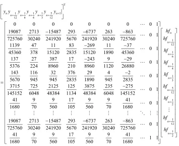
m n n m
Y ey hdf y hdf Y (8)
where , ,are e d r r matrix
where
T
19087 1139 137 143 3715 41
725760 45360 5376 5670 145152 1680
d
T
1 1 1 1 5 1
12 6 4 3 12 2
, , ,
, ,
m
n n n n n n
Y y y y y y y
0 0 0 0 0 1 0 0 0 0 0 1 0 0 0 0 0 1 0 0 0 0 0 1 0 0 0 0 0 1 0 0 0 0 0 1
e
5 t
2713 15487 293 6737 263 863
30240 241920 5670 241920 30240 725760
47 11 83 269 11 37
378 15120 2835 15120 1890 45360
27 387 17 243 9 29
224 8960 210 8960 1120 26880
116 32 376 29 4 2
945 945 2835 1890 945 2835
725 2125 125 3875
6048 48384 1134 4
b
235 275
8384 6048 145152
9 9 17 9 9 41
70 560 105 560 70 1680
3. Analysis of the Basic Properties of Our
New Method
3.1. Order of the Method
Let the linear operator L y x
:h
associated with the block formular be defined as
:
0
m n n m
L y x h A Y ey h df y h bF Y
(9) expanding in Taylor series and comparing the coeffi- cient of h gives
0 1 1
1 1 2 2
1 2
; x x p p
p
p p p p
p p
L y x h c y x c hy c hy c h y x
c h y x c h y
(10) Definition:-The linear operator L and the associated
continuous linear multistep method (3.1) are said to be of o r d e r p i f c0 c1c2 cp 0 and cp10 i s
called the error constant and implies that the local trun-cation error is given by
1 1 2
2 0 .
p p p
n k p n
t C h y x h
For our method;
1 1 12 12 1 1 6 6 1 1 4 4 1 1 3 3 5 5 12 12 1 1 2 2 1 1 12 1 1 6 1 1 4 ; 1 1 3 5 1 12 1 1 2 n n n n n n n n n n n n n n f h y f h y f y h fL y x h y
y h f y f h y f h 0
Expanding in Taylor series expansion gives
1 1
0 0
1
19087 2713 1 15487 1
12
! 725760 ! 30240 12 241920 6
293 1 6737 1 263 5 863 1
5670 4 241920 3 30240 6 725760 2
j
j j
j
j j
n n n n
j j
j j j j
h
y y hy y
j j
1 1 0 0 11139 47 1 11 1
6
! 45360 ! 378 12 15120 6
83 1 269 1 11 5 37 1
2835 4 15120 3 1890 12 45360 2
j
j j
j
j j
n n n n
j j
j j j j
h
y y hy y
j j
0 1 1 0 1137 27 1 387 1
4
! 5376 ! 224 12 8960 6
17 1 243 1 9 5 29 1
210 4 8960 3 1120 12 26880 2
j
j j
j
j j
n n n n
j j j
j j
j
h
y y hy y
j j
1 1 0 0 1143 116 1 32 1
3
! 5670 ! 945 12 945 6
376 1 29 1 4 5 2 1
2835 4 1890 3 945 12 2835 2
j
j j
j
j j
n n n n
j j j
j j
j
h
y y hy y
0
1 0
1
5
3715 725 1 2125 1
12
! 145152 ! 6048 12 48384 6
125 1 3875 1 235 5 275 1
1134 4 48384 3 6048 12 145152 2
j
j j
j
j j
n n n n
j j
j j j j
h
y y hy y
j j
1
0 0
1
1
41 9 1 9 1
2
! 1680 ! 70 12 560 6
17 1 9 1 9 5 41 1
105 4 560 3 70 12 1680 2
j
j j
j
j j
n n n n
j j j
j j
j
h
y y hy y
j j
Equating coefficients of the Taylor series expansion to zero yield
0 1 6 0
c c c
Hence we arrived at a uniform order 6 for our method with error constants
7 3.78 09 2.53 09 3.49 09 1.85 09 1.68 08 5.56 08
c
3.2. Zero Stability
Definition: The block (8) is said to be zero stable, if the roots Zs, s1, 2, , N
of the characteristic polynomial
defined by satisfies
z
0det
z zA E
exceeding the order of the differential equation. More-over as 0,
r
1
h z z z where is the order of the differential equation, r is the order of the matrix A 0 and E.
zs 1and every root satisfying zs 1 have multiplicity not For our method
1 0 0 0 0 0 0 0 0 0 0 1
0 1 0 0 0 0 0 0 0 0 0 1
0 0 1 0 0 0 0 0 0 0 0 1
0
0 0 0 1 0 0 0 0 0 0 0 1
0 0 0 0 1 0 0 0 0 0 0 1
0 0 0 0 0 1 0 0 0 0 0 1
z z
5
1 .
z z z
Hence our method is zero stable.
3.3 Region of Absolute Stability
The block formulated as a general linear method where it is partition in the form
1 1
2 2
n i n
Y A B hf y
Y A B y
The elements of A1 and A2 are obtained from the
coefficients of the collocation points, and are obtained from the interpolation points. 1
B B2
Applying the test equation y y leads to the re-
currence equation
1 , , 1, 2, , 1
i i
y M Z y Z h i
The stability function is given by
12 2 1
B M Z B ZA IZA
and the stability polynomial of the method is given as
,Z
det
I M Z
The region of absolute stability of the method is de- fined as
,Z
1, 1.T
1 1 1 1 5 1 12 6 4 3 12
0 0 0 0 0 0 0 0 1
19087 2713 15487 293 6737 263 863 0 1
725760 30240 241920 5670 241920 30240 725760
1139 47 11 83 269 11 37
0 1
45360 378 15120 2835 15120 1890 45360
137 27 387 17
5376 224 8960 210
n n
n n n n n
y y y y y y y
243 9 29 0 1
8960 1120 26880
143 116 32 376 29 4 2
0 1
5670 945 945 2835 1890 945 2835
3715 725 2125 125 3875 235 275 0 1
145152 6048 48384 1134 48384 6048 145152
41 9 9 17 9 9 41 0 1
1680 70 560 105 560 70 1680
19087 2713 15487
725760 30240 2
1 12 1 6 1 4 1 3 5 12 1 2
1 12 1 2
293 6737 263 863 0 1
41920 5670 241920 30240 725760
41 9 9 17 9 9 41
1 1
1680 70 560 105 560 70 1680
n
n
n
n
n
n
n
n
n
hf hf
hf
hf
hf
hf
hf
hf
hf
4. Real Life Problems
4.1. Problem 1: (SIR MODEL)
The SIR model is an epidemiological model that com- putes the theoretical numbers of people infected with a contagious illness in a closed population over time. The name of this class of models derives from the fact that they involves coupled equations relating the number of susceptible people S(t), number of people infected I(t) and the number of people who have recovered R(t). This is a good and simple model for many infectious diseases including measles, mumps and rubella [13-15]. The SIR model is described by the three coupled equations.
d 1 d
s
S I
t S (11)
d d
I
I I I
t S (12)
d d
s R
t I (13)
where , and are positive parameters. Define to be
y
y S I R
(14) Adding Equations (11)-(13), we obtain the following evolution equations for
y
1
y
Taking 0.5 and attaching an initial condition
0y 0.5 (for a particular closed population), we ob-
tain,
0.5 1
, 0 0.5y t y y (16)
whose exact solution is,
1 0.5e0.5ty t (17)
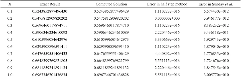
Applying our new half step numerical scheme (8) to solve SIR model simplified as (17) gives results as shown in Table 1.
4.2. Problem 2 (Growth Model)
Let us consider the differential equation of the form;
d , 0 1000, 0,1
d
N
N N t
t (18)
Equation (18) represents the rate of growth of bacteria in a colony. We shall assume that the model grows con- tinuously without restriction. One may ask; how many bacteria are in the colony after some minutes if an indi- vidual produces an offspring at an average growth rate of 0.2? We also assume that N t
is the population size attime (t Table 2).
The theoretical solution of (18) is given by;
s (19)
[image:6.595.121.476.85.374.2]Table 1. Showing results for SIR model problem.
X Exact Result Computed Solution Error in half step method Error in Sunday et al.
[image:7.595.54.546.288.446.2]0.1 0.5243852877496430 0.5243852877496429 1.110223e−016 5.574430e−012 0.2 0.5475812909820202 0.5475812909820202 0.000000e+000 3.946177e−012 0.3 0.5696460117874711 0.5696460117874710 1.110223e−016 8.183232e−012 0.4 0.5906346234610092 0.5906346234610089 2.220446e−016 3.436118e−011 0.5 0.6105996084642976 0.6105996084642973 3.330669e−016 1.929743e−010 0.6 0.6295908896591411 0.6295908896591410 1.110223e−016 1.879040e−010 0.7 0.6476559551406433 0.6476559551406429 4.440892e−016 1.776835e−010 0.8 0.6648399769821805 0.6648399769821799 5.551115e−016 1.724676e−010 0.9 0.6811859241891134 0.6811859241891132 2.220446e−016 1.847545e−010 1.0 0.6967346701436834 0.6967346701436828 5.551115e−016 3.005770e−010
Table 2. Showing results for growth model problem.
X Exact Result Computed Solution Error in half step method Error in Sunday et al.
0.1 1020.2013400267558 1020.201340026755 0.000000e+000 1.830358e−011 0.2 1040.8107741923882 1040.8107741923882 0.000000e+000 1.250555e−011 0.3 1061.8365465453596 1061.8365465453596 0.000000e+000 1.227818e−011 0.4 1083.2870676749587 1083.2870676749585 2.273737e−013 3.137757e−011 0.5 1105.1709180756477 1105.1709180756475 2.273737e−013 2.216893e−010 0.6 1105.1709180756477 1127.4968515793755 2.273737e−013 2.060005e−010 0.7 1150.2737988572273 1150.2737988572271 2.273737e−013 2.171419e−010 0.8 1173.5108709918102 1173.5108709918102 0.000000e+000 2.216893e−010 0.9 1197.2173631218102 1197.2173631218102 0.000000e+000 2.744400e−010 1.0 1221.4027581601699 1221.4027581601699 0.000000e+000 4.899903e−010
Applying our new half step numerical scheme (8) to solve the Growth model (17) gives results as shown in
Table 2 [16].
4.3. Problem 3 (Decay Model)
A certain radioactive substance is known to decay at the rate proportional to the amount present. A block of this substance having a mass of 100 g originally is observed. After 40 mins, its mass reduced to 90 g. Find an expres- sion for the mass of the substance at any time and test for the consistency of the block integrator on this problem for t
0,1 .The problem has a differential equation of the form;
d , 0 100, 0,1
d
N
N N t
t (21)
where N represents the mass of the substance at any time
and
t is a constant which specifies the rate at which
this particular substance decays. Note that,
0 100 g, 40 mins, 40
90 gf t f
0 e tf t f 40
90 100e
ln 9 ln10
0.0026 40
Thus, the theoretical solution to (20) is given by,
100e 0.0026tf t (22)
which is also the expression for the mass of the substance at any time t.
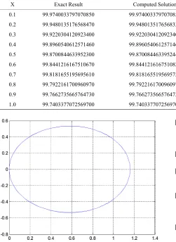
Applying our new half step numerical scheme (8) to solve the Growth model (22) gives results as shown in
Table 3 [16,17] (Table 3).
5. Discussion of the Result
We have considered three real-life model problems to test the efficiency of our method. Problems 1 and 2 and 3 were solved by Sunday et al. [17]. They proposed an
Table 3. Showing results for decay model problem.
X Exact Result Computed Solution Error in half step method Error in Sunday et al.
0.1 99.9740033797070850 99.9740033797070850 0.000000e+000 0.000000e+000 0.2 99.9480135176568470 99.9480135176568330 1.421085e−014 1.421085e−014
0.3 99.9220304120923400 99.9220304120923400 0.000000e+000 0.000000e+000 0.4 99.8960540612571460 99.8960540612571460 0.000000e+000 0.000000e+000 0.5 99.8700844633952300 99.8700844633952440 1.421085e−014 0.000000e+000 0.6 99.8441216167510670 99.8441216167510820 1.421085e−014 0.000000e+000 0.7 99.8181655195695610 99.8181655195695750 1.421085e−014 0.000000e+000 0.8 99.7922161700960970 99.7922161700960970 0.000000e+000 0.000000e+000 0.9 99.7662735665764730 99.7662735665764730 0.000000e+000 0.000000e+000 1.0 99.7403377072569700 99.7403377072569700 0.000000e+000 0.000000e+000
Figure 1. Showing region of absolute stability of our method.
1-3 because the iteration per step in the new method was
lower than the method proposed by [17]. Our method was found to be zero stable, consistent and converges.
Figure 1 shows the region of absolute stability. From the
numerical examples, we could safely conclude that our method gave better accuracy than the existing methods.
REFERENCES
[1] A. O. Adesanya, M. R. Odekunle, and A. A. James, “Or- der Seven Continuous Hybrid Methods for the Solution of First Order Ordinary Differential Equations,” Canadian Journal on Science and Engineering Mathematics, Vol. 3
No. 4, 2012, pp. 154-158.
[2] A. M. Badmus and D. W. Mishehia, “Some Uniform Or- der Block Methods for the Solution of First Ordinary Dif- ferential Equation,” J. N.A.M. P, Vol. 19, 2011, pp 149- 154.
[3] J. Fatokun, P. Onumanyi and U. W. Sirisena, “Solution of First Order System of Ordering Differential Equation by Finite Difference Methods with Arbitrary,” J.N.A.M.P, 2011, pp. 30-40.
[4] B. I. Zarina and S. I. Kharil, “Block Method for General- ized Multistep Method Adams and Backward Differential Formulae in Solving First Order ODEs,” MATHE-MATIKA, 2005, pp. 25-33.
[5] G. Dahlquist, “A Special Stability Problem for Linear Multistep Methods,” BIT, Vol. 3, 1963, pp. 27-43. [6] P. Onumanyi, U. W. Sirisena and S. A. Jator, “Solving
Difference Equation,” International Journal of Comput- ing Mathematics, Vol. 72, 1999, pp. 15-27.
[7] E. A. Areo, R. A. Ademiluyi and P. O. Babatola, “Three- Step Hybrid Linear Multistep Method for the Solution of First Order Initial Value Problems in Ordinary Differen- tial Equations,” J.N.A.M.P, Vol. 19, 2011, pp. 261-266. [8] E. A. Ibijola, Y. Skwame and G. Kumleng, “Formation of
Hybrid of Higher Step-Size, through the Continuous Mul- tistep Collocation,” American Journal of Scientific and Industrial Research, Vol. 2, 2011, pp. 161-173.
[9] H. S. Abbas, “Derivation of a New Block Method Similar to the Block Trapezoidal Rule for the Numerical Solution of First Order IVPs,” Science Echoes, Vol. 2, 2006, pp.
10-24.
[10]Y. A. Yahaya and G. M. Kimleng, “Continuous of Two- Step Method with Large Region of Absolute Stability,” J.N.A.M.P, 2007, pp. 261-268.
[11]A. O. Adesanya, M. R. Odekunle and A. A. James, “Start- ing Hybrid Stomer-Cowell More Accurately by Hybrid Adams Method for the Solution of First Order Ordinary Differential Equation,” European Journal of Scientific Research, Vol. 77 No. 4, 2012, pp. 580-588.
[12]S. Abbas, “Derivations of New Block Method for the Nu- merical Solution of First Order IVPs,” International Jour- nal of Computer Mathematics, Vol. 64, 1997, p. 325.
[13]W. B. Gragg and H. J. Stetter, “Generalized Multistep Predictor-Corrector Methods,” Journal of Association of Computing Machines, Vol. 11, No. 2, 1964, pp. 188-209.
http://dx.doi.org/10.1145/321217.321223
[14]J. B. Rosser, “A Runge-Kutta Method for All Seasons,”
SIAM Review, Vol. 9, No. 3, 1967, pp. 417-452.
http://dx.doi.org/10.1137/1009069
[16] O. D. Ogunwale, O. Y. Halid and J. Sunday, “On an Al- ternative Method of Estimation of Polynomial Regression Models,” Australian Journal of Basic and Applied Sci- ences, Vol. 4, No. 8, 2010, pp. 3585-3590.
[17] J. Sunday, M. R. Odekunleans and A. O. Adeyanya, “Or der Six Block Integrator for the Solution of First-Order Ordinary Differential Equations,” IJMS,Vol. 3, No. 1 2013,