Multiple Testing Techniques in Growth Econometrics

(1)

Munich Personal RePEc Archive

Multiple Testing Techniques in Growth

Econometrics

Deckers, Thomas and Hanck, Christoph

Universität Bonn, Rijksuniversiteit Groningen

10 October 2009

Online at

https://mpra.ub.uni-muenchen.de/17843/

(2)

Multiple Testing Techniques in Growth Econometrics

∗

Thomas Deckers† Universit¨at Bonn

Christoph Hanck‡ Rijksuniversiteit Groningen

October 13, 2009

Abstract

This paper discusses two longstanding questions in growth econometrics which involve multiple hypothesis testing. In cross sectional GDP growth regressions many variables are simultane-ously tested for significance. Similarly, when investigating pairwise convergence of output for

n countries, n(n−1)/2 tests are performed. We propose to control the false discovery rate (FDR) so as not to erroneously declare variables significant in these multiple testing situations only because of the large number of tests performed. Doing so, we provide a simple new way to robustly select variables in economic growth models. We find that few other variables beyond the initial GDP level are needed to explain growth. We also show that convergence of per capita output using a time series definition with the necessary condition of no unit root in the log per-capita output gap of two economies does not appear to hold.

Keywords: Growth Empirics, Multiple Testing, Convergence, Bootstrap

JEL-Codes: O47, C12

∗_{We thank Franz Palm, Stephan Smeekes and Jean-Pierre Urbain for useful comments that helped improve the}

paper. Part of the paper was written while the authors were at Maastricht University, whose hospitality is gratefully acknowledged. All errors are ours. The data and programs used in this paper are available upon request.

†_{Department of Economics,}

[email protected].

‡_{Department of Economics and Econometrics, Nettelbosje 2, 9747AE Groningen, Netherlands. +31 (0)50 363}

(3)

1 Introduction

Why do some countries grow faster than others? What determines long-run economic growth? These intriguing questions have been part of economic research since its beginnings. Answering them would permit more stable, long-run oriented policy making. Moreover, knowing what truly determines growth would help tackle the inequality in living standards between countries. The importance of this issue is reflected in the extensive research in this area. Unfortunately, different authors find quite diverse components to determine economic growth (Durlauf, Kourtellos and Tan, 2008). A far from exhaustive list includes initial GDP, fertility rates, high school enrolment rates, public debt and quality of institutions.

In judging whether a variable is significant in an economic growth model, researchers often rely on traditional significance tests. That is, one tests each coefficient individually at some level α using appropriate p-values. Given the large set of possible explanatory variables in a growth regression, one simultaneously tests a large number of hypotheses. Given someα, the probability of committing at least one type I error is arbitrarily larger thanα. To see this, note the event of a rejection is a Bernoulli random variable with “success” probabilityα if the null is true. Hence, assuming (for illustration only) that all hypotheses are true and independent, Pl, the probability

of finding l rejections in k tests, corresponding to k possible regressors, is the probability mass function of a Binomial random variable,

Pl=

k l

!

αl(1₋α)k−l.

Therefore, the probability of at least one erroneous rejection forα= 0.05 and k= 50 equals

Pl>1= 50

X

j=1

50 j

!

0.05j(1₋0.05)50−j = 0.9231.

Hence, one is bound to erroneously declare irrelevant variables to explain growth. This is of substantial policy relevance. Growth regressions are used to identify effective policy measures to boost growth. Now, if variables are only spuriously found related to growth, ineffective public expenditures may well arise.

The issue is thus related to, but different from, data mining, where, in the words of Lovell (1983) “a data miner uncovers t-statistics that appear significant at the 0.05 level by running a large number of alternative regressions on the same body of data.” Doing so, “the probability of a type I error of rejecting the null hypothesis when it is true is much greater than the claimed 5%.”

Another topic extensively researched in growth econometrics is whether per-capita outputs of different economies converge. Investigating convergence is relevant for example in the context of European integration. Of the different notions of convergence proposed in the literature1 _we

will focus on convergence across economies using a time-series definition proposed by Pesaran (2007). There, two economies converge only if a unit root test on the output gap of two economies,

(4)

i.e. the difference of the log per-capita income, rejects. These pairwise tests with the null of no convergence are conducted for all different combinations ofncountries. This results inn(n₋1)/2 simultaneous tests. Again, given the high number of simultaneous tests, even if no country pair converges one is bound to falsely reject the null of no convergence for several pairs.

We propose to tackle these problems by using multiple testing techniques. These take the mul-tiplicity of tests performed explicitly into account. One way to achieve such mulmul-tiplicity control is to only declare a variable significant if its p-value satisfies pj 6 αj for some suitably chosen

cutoff αj 6 α. Such multiple testing techniques are routinely applied in many areas of applied

statistics that involve multiple hypothesis testing, e.g. genomics (e.g., Dudoit and van der Laan, 2007). Following Romano, Shaikh and Wolf (2008b), we argue that selecting important regressors in this fashion can fruitfully be used as a simple-to-use model selection device. In that way, we aim to find a new way to robustly select explanatory variables in economic growth models and to shed some further light on the question whether economies converge.

We will focus on controlling the False Discovery Rate (FDR) (Benjamini and Hochberg, 1995). The FDR is defined as the expected value of the number of falsely rejected hypotheses divided by the overall number of rejections. It is thus an extension of the notion of a type I error to the multiple testing situation. For the first application, rejection means declaring some determinant to be significant in an economic growth model. In the second application, rejection means rejection of the null of no convergence.

The rejective power of the FDR controlling procedures might differ substantially (Romano, Shaikh and Wolf, 2008a). Thus, we first conduct an extensive Monte Carlo study judging the effectiveness of the procedures under different settings relevant to the present testing problems.

We find that few other variables beyond initial GDP level are needed to explain growth. We also show that output convergence using a time series definition with the necessary condition of no unit root in the output gap of two economies does not seem to hold.

This paper is organized as follows. Section 2 surveys previous approaches in cross-sectional growth models as well as in the convergence literature. Section 3 describes the FDR controlling procedures that we employ. Section 4 assesses their quality in a Monte Carlo study. Section 5 examines cross sectional growth regressions using FDR controlling techniques and compares the results to other approaches used in the literature. Section 6 conducts FDR controlling pairwise tests for output convergence. The final section concludes.

2 Literature Review

2.1 Growth Regressions

(5)

a specification is consistent with a variety of neoclassical growth models that have as possible solution a log-linearization around the steady state of the form (Barro and Sala-i-Martin, 1995)

logyT −logy0 =−(1−e−λT) logy0+ (1−e−λT) logy∗, (1)

where logyt is the logarithm of the per capita gross domestic product (GDP for short) at time

t, logy∗ _{is its steady-state value, and} _λ _{is the convergence rate. If all economies have the same}

steady state, the regression corresponding to (1) forncountries and time periodsT and 0 reads:

log(yiT/yi0) =µ+δlog(yi0) +ui, i= 1, . . . , n, (2)

whereui is a disturbance term. Here,δ is expected to have a negative sign, indicating that poor

economies tend to grow faster and converge to rich ones. This is calledabsolute convergence(Barro and Sala-i-Martin, 1995). But when taking (2) to the data, this effect can only be seen when fitting the regression to a set of relatively homogeneous economies. This is because economies generally differ in their steady state. For heterogeneous economies, the sign ofδbecomes ambiguous (Barro and Sala-i-Martin, 1995). The reason is that heterogeneous economies have different individual-specific parameters that determine their steady states. Omitting these from (2) leads to a bias. This motivates the concept of conditional convergence. To incorporate this into (2), one adds additional control variables xi, measuring the steady state determinants of an economy. The

equation then becomes:

log(yiT/yi0) =µ+δlog(yi0) +x′iβ+ui, i= 1, . . . , n, (3)

Although specifications like (3) are very widely used in the literature, there is little agreement on which variables to include in the vectorxi.

Barro (1991) performs growth regressions with data for 98 countries from 1960 to 1985. Next to the negative relation to initial GDP, he finds a positive relation of growth to initial human capital. Furthermore, growth appears to be inversely related to the share of government consumption and a proxy for market distortions, but positively related to measures of political stability. Following this seminal work, the literature pointed out many different variables that would be significant in explaining growth. However, few authors perform multiplicity control in spite of often using a number of candidate variables of the same order of magnitude asn.

(6)

this model uncertainty, Sala-i-Martin et al. (2004) find 11 variables to robustly explain growth, of which initial GDP level again has the strongest impact. The related work of Durlauf et al.

(2008) aims at finding relevant growth theories rather than single variables. The results are still comparable to the aforementioned papers in that they declare a growth theory to be important if at least one variable associated with that theory appears in the final model. The reliability of these studies using BMA is questioned in Ley and Steel (2009). They show that the choices made concerning prior distributions strongly affect the number of variables declared significant. Thus the results are sensitive to difficult and somewhat subjective user choices.

2.2 Pairwise Testing for Output Convergence

The literature discusses different definitions for output convergence and resulting tests; see Islam (2003) for a survey. We are concerned with pairwise output convergence across countries. We work with the time-series definition of Pesaran (2007). He assumes the following common factor model for the GDP of countryi at timet,yit,2

yit=ci+git+θi′ft+ǫit+ηit fori= 1,2, . . . , n. (4)

Here,ηit is a zero-mean stationary process, but ft and ǫit could be non-stationary. Following the

definition in Bernard and Durlauf (1995), countries iandj converge if

lim

k→∞E(yi,t+k−yj,t+k|Ft) = 0 at any fixed timet, (5)

where Ft is an information set containing at least the current and past output series yi,t−s for

i = 1,2, . . . , n and s = 1,2, . . . , t. Bernard and Durlauf (1995) show that for (5) to hold, a necessary, though not sufficient, condition is that the GDPs are cointegrated with cointegrating vector (1,₋1)′_{. Substituting (4) into (5) the condition for convergence reads}

lim

k→∞(ci−cj) + (gi−gj)(t+k) + (θi−θj) ′_E(_f

t+k|Ft) +

E(ǫi,t+k−ǫj,t+k|Ft) + E(ηi,t+k−ηj,t+k|Ft) = 0.

Since ηit is assumed to be stationary, so is the differenceηit−ηjt. Thus, we have

lim

k→∞E(ηi,t+k−ηj,t+k|Ft) = E(ηit−ηj,t) = 0.

Moreover, for convergence it has to hold that ǫit is I(0), since otherwise limk→∞E(ǫi,t+k −

ǫj,t+k|Ft) 6= 0. We now have to consider two cases for the order of integration of θ′ift, namely

θ_i′ft∼I(0) andθi′ft∼I(1). Under the former, convergence according to (5) requires thatci =cj

and gi=gj. Ifθ′ft∼I(1) we must also have thatθi=θj.

Pesaran (2007) argues that of these three conditions, the most unlikely to hold is ci = cj. This

would require the two converging countries to be identical in nearly every respect, including for example their initial endowment. Hence, he employs a less stringent definition of convergence.

(7)

The definition is based on the idea that for two countries i and j to converge, the output gap yit−yjt should not fall outside a pre-specified interval C with high probabilityπ. Formally,

Pr_{|yi,t+s−yj,t+s|< C|Ft}> π, (6)

for alls= 1,2, . . . ,_∞. This less stringent definition of pairwise convergence requiresyit−yjt not

to have a stochastic or deterministic trend. But contrary to (5), (6) does not require ci =cj for

two countries to converge.

Using a cointegration framework and (6), the GDPs of two countriesiandjshould be cointegrated and cotrended with vectors (1,₋1)′ _{for them to converge. Pesaran (2007) demonstrates that this}

condition can be checked by directly testing each output gap for the absence of a unit root and a linear trend. In this setting, the absence of a unit root can be seen as a necessary condition and the additional absence of a linear trend (gi =gj) as a sufficient condition.

Pesaran (2007) tests for the absence of a unit root for all possible n(n₋1)/2 pairs of countries. For largenandT, if no country pair converges, the null of no convergence should only be rejected for a fraction of pairs equal to the significance levelα of the individual tests applied. In this case, the null could have been rejected by chance for pairs found to be convergent. On the other hand, if all country pairs converge, for large n and T, the fraction of country pairs found convergent should tend to 1. Using data from the Penn World Tables 6.1 he only rejects the null for a fraction of country pairs roughly equal toα. Hence, he finds no evidence for overall convergence. However, since his approach makes no statements about individual country pairs it cannot say whether the fraction of rejections consists entirely of type I errors or possibly does contain some correct rejections.

Further studies using a time-series framework and similar definitions of convergence are also largely in disfavor of the overall convergence hypothesis. Bernard and Durlauf (1995) apply cointegration tests in a panel setting to test for convergence. They fail to find convergence for a set of 15 OECD countries when testing for the cointegration vector (1,₋1)′. Nevertheless they find cointegration relationships of the form (1,₋a) among different countries. This indicates, following their definition, conditional convergence, a concept less strict than the one employed here. Pesaran (2007) shows that this approach can only handle a limited number of countries simultaneously. Earlier studies using univariate time series techniques (e.g., Campbell and Mankiw, 1989; Quah, 1990) also fail to find evidence for overall convergence. A problem inherent to their approaches is the choice of a ‘reference country’ to which convergence of the other economies is tested.

(8)

3 Controlling the FDR

The false discovery rate (FDR) as a desirable measurement of type I errors in multiple testing situations is introduced by Benjamini and Hochberg (1995). They also provide a step-up procedure that is shown to control the FDR at a desired levelγ. A step-up method considers the hypotheses ordered from most significant to least significant based on their p-values. The idea is then, beginning with the least significant hypothesis, to accept hypotheses up to a certain point and reject the remaining ones.

We now present four methods controlling the FDR in more detail. Concretely, we employ the methods from Benjamini and Hochberg (1995), Storey, Taylor and Siegmund (2004), Benjamini, Krieger and Yekutieli (2006) and the bootstrap method of Romano et al. (2008a). We will frequently refer to these as BH method, Storey method, BKY algorithm and bootstrap method.

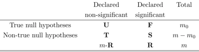
Adapting a notation similar to Benjamini and Hochberg (1995) and referring to Table 1, there are m hypotheses to be tested simultaneously out of which m0 are true. R is an observable random

variable, whereas U, F, S and T are unobservable random variables. The proportion of falsely rejected null hypotheses can be described by Q =F/(F+S). Naturally, if F+S = 0, we take

Q= 0. The FDR is then defined as E(Q) = E(F/(F+S)) = E(F/R). Lower-case letters denote the realizations of the underlying random variable.

3.1 BH Method

In the FDR controlling method suggested in Benjamini and Hochberg (1995) one first chooses a level γ at which to control the FDR. Let p_b₍₁₎ _≤ . . . _≤ p_b₍_m₎ be the ordered p-values and H₍₁₎, . . . , H₍_m₎the corresponding null hypotheses, such that the hypotheses are now ordered from most to least significant. For 1 _≤j _≤m, let γj = _mjγ. Then the method rejects H(1), . . . , H(j∗₎,

where j∗ _{is the largest}_j _{such that} b

p₍_j₎ _≤ γj. If no suchj exists, no hypothesis is rejected. The

intuition behind the procedure is the following: When testing each hypothesis at some level α, we have that E(F) _≤αm. So a valid estimate for the upper bound of the expected value of Q

[image:8.595.142.463.634.718.2]

isαm/r(α), where r(α) denotes the number of rejected hypotheses when testing each at levelα. Given the observedp-values, αcan now be chosen to maximize the observed number of rejections r(α) given the constraint that FDR _≤γ. Given FDR _≤γ, maximizing the observed number of

Table 1: Number of decisions made when testingm null hypotheses Declared Declared Total non-significant significant

True null hypotheses U F m0

Non-true null hypotheses T S m₋m0

(9)

rejections is desirable, since this identifies as many false hypotheses as possible. Here this means that one finds as many relevant variables as possible. Moreover, Benjamini and Yekutieli (2001) show control of the FDR under positive regression dependency, which under certain conditions includes coefficient test statistics in static regressions. The Monte Carlo study in section 4 shows that the FDR is also controlled under plausible assumptions about e.g. the DGP of a cross-sectional growth regression.

3.2 Storey Method

Even if the conditions of the BH method are met the method is conservative as it can be shown that FDR _≤ m0

mγ. So, unlessm0 = m, the power of the method can be improved by redefining

γj as γj = _mj₀γ. Since m0 is unknown, it has to be estimated. Storey et al. (2004) propose to

estimate m0 by mb0 = #[bp₁j>λ₋_λ]+1, where λ∈(0,1) is a user-specified parameter. The idea behind

this estimator is the following: p-values corresponding to true null hypotheses approximately follow a uniform[0,1] distribution. Therefore one would expect m0(1−λ) of these to lie in the

interval (λ,1]. When replacing m in the BH method by ˆm0, Storeyet al. (2004) show that this

procedure typically controls the FDR whenever the BH method does. The Storey procedure can however be quite liberal under constant positively dependentp-values.

3.3 BKY Algorithm

Benjaminiet al.(2006) propose another improvement of the original BH method. It comes in the form of a two step algorithm. First, one applies the BH procedure at a level γ∗ ₌_{γ/(1 +}_γ_{). If}

r = 0, no hypothesis is rejected and the procedure stops. Likewise, if r =m, all hypotheses are rejected. Otherwise, the procedure continues using the BH method with γj replaced by _m_ˆj₀γ∗,

where ˆm0 =m−r. Benjaminiet al.(2006) prove that this method works under independent test

statistics and also provide simulations suggesting that it works under dependent test statistics.

3.4 Bootstrap Method

The bootstrap method is a step-down rather than a step-up procedure as the three previously described methods. Assume without loss of generality that a hypothesisH₍_i₎ is rejected for large values of its corresponding test statistic Ti. Further, order the test statistics from smallest to

largest, i.e.T1≤T2 ≤. . .≤Tm, and letH(1), H(2), . . . , H(m)denote the corresponding hypotheses.

A step-down procedure then compares the largest test statistic Tm with a suitable critical value

cm. IfTm< cm the procedure rejects no hypothesis; otherwise it rejectsH(m) and steps down to

Tm−1. The procedure continues in this fashion until it either rejectsH(1) or does not reject the

current hypothesis. More formally, a step-down procedure rejects hypotheses

(10)

wherej∗ _{is the largest integer}_j _satisfying

Tm ≥cm, Tm−1 ≥cm−1, . . . , Tm−j ≥cm−j.

If no suchj exists, the method does not reject any hypotheses.

3.4.1 Intuition

Recall the FDR is the expected value of falsely rejected hypotheses over the total number of rejected hypotheses. For any step-down procedure this expected value can be calculated as

FDR = E

_F

max_{R,1_}

= X

1≤r≤m

1

rE[F|R=r]P{R=r}

= X

1≤r≤m

1

rE[F|R=r]

×P_{Tm ≥cm, . . . , Tm−r+1 ≥cm−r+1, Tm−r< cm−r},

where the event Tm−r < cm−r is defined to be true when r=m.

Assume without loss of generality that the true hypotheses correspond to the indices_{1, . . . , m0}.

Under weak assumptions relating to test consistency, all other (i.e. the false) hypotheses are rejected with probability tending to one. Moreover, let Tr:t denote the rth smallest of the test

statistics T1, . . . , Tt. In particular, when t= m0, Tr:m0 denotes the rth smallest test statistic of

all true hypotheses. Then, with probability approaching one,

FDR = X

m−m0+1≤r≤m

r₋m+m0

r (7)

×P_{Tm0:m0 ≥cm0, . . . , Tm−r+1:m0 ≥cm−r+1, Tm−r:m0 < cm−r}.

Again the event Tm−r < cm−r is defined to be true when r = m. The intuition behind (7) is

the following: Given that all false hypotheses are rejected with probability tending to one, one only needs to search among the hypotheses_{H1, . . . , Hm0}how many of these are falsely declared

significant. Then, summing over every possible proportion of falsely rejected hypotheses weighted by its probability gives the expected value of this, i.e. the FDR.

Since m0 is unknown, one has to ensure that (7) is bounded above by γ for every possible m0.

That is exactly the condition used to recursively determine the critical values. For m0 = 1, (7)

simplifies to

FDR = 1

mP{T1:1 ≥c1}. Hence one can calculate the first critical value from

c1 = inf

x_∈R: 1

mP{T1:1 ≥x} ≤γ

Ifmγ >1,c1 is set to−∞. Form0 = 2, (7) equals

1

m₋1P{T2:2≥c2, T1:2 < c1}+ 2

(11)

Hence, having determined c1, c2 then simply is the smallest number for which (8) is bounded

above by γ. In general, having determined c1, . . . , cj−1, cj is the smallest value for which the

following expression is bounded above byγ,

FDR = X

m−j+1≤r≤m

r₋m+j r

×P_{Tj:j ≥cj, . . . , Tm−r+1:j ≥cm−r+1, Tm−r:j < cm−r} (9)

Forj =m, (9) simplifies to

P_{Tm:m ≥cm}.

Thus, one can find the mth critical value via the following minimization:

cm = inf{x∈R:P{Tm:m≥x} ≤γ}.

In practice this choice of critical values is infeasible, since the probability measureP is unknown. Hence,P is approximated using bootstrap techniques as presented in the following.

3.4.2 Procedure

The idea is to replaceP by a suitable ˆP using bootstrap techniques. The exact choice of bootstrap depends of course on the nature of the data and the problem that is analyzed. We will present the two bootstrap procedures used later. Here, it is only required that ˆP estimatesP such that T∗

j, the bootstrapped test statistic, is a good approximation of Tj whenever the corresponding

null hypothesis is true (Romanoet al., 2008a).

Given ˆP, the critical values are defined recursively as follows: Having determined ˆc1, . . . ,ˆcj−1, the

jth critical value is determined using the minimization rule (Romanoet al., 2008a):

ˆ

cj = inf

c_∈_R: X

m−j+1≤r≤m

r₋m+j

r (10)

×PˆT_j∗_:_j _≥c, . . . , T_m∗₋_r_+1:_j _≥cˆm−r+1, Tm∗−r:j <ˆcm−r ≤γ

Here, it is crucial to understand the meaning of T∗

r:t. The index t stems from the ordering of

the original test statistics, whereas r corresponds to the bootstrapped test statistics. So T∗

r:t has

the following meaning: Out of the t smallest original test statistics pick the rth smallest of the corresponding bootstrap test statistics.

3.4.3 Linear Regression Model

For the application to cross sectional growth regressions we consider the model

y=Xβ+u,

(12)

1. Estimateβ using ˆβ= (X′X)−1_X′_y_.

2. Calculate the residuals ûusing û=y₋Xβând their demeaned version ˜u= û₋ι(ι′ι)−1_ι′_u_ˆ_,

whereιis a vector of ones.

3. For each element ofβ, calculate the t-statistic _√ βˆi

s2₍_X′_X₎−1

ii

for H0: βi= 0 against H1: βi6=

0. Here s2 =P_i ˆu2i

n−(k+1).

4. Resample non-parametrically with replacement from ˜uto obtain the bootstrap residualsu∗

i

and build the bootstrap sample

y_i∗ =x′_iβˆ+u∗_i 5. Calculate ˆβ∗ = (X′X)−1_X′_y∗ _and _u∗ ₌_y∗₋_X_β_ˆ∗_.

6. For each element of ˆβ∗ construct the bootstrapped version of each individual t-statistic using the formula βˆ∗i−βˆi

√

s2∗₍_X′_X₎−1

ii

, wheres2∗ ₌P

i u∗2

i

n−(k+1). Repeat steps 4 – 6 B times.

7. Apply the rule (10) with m=k+ 1 to calculate the critical values.

8. Use the critical values from 7 and compare them in the previously described step-down fashion (10) to the t-statistics found in 2.

We thus bootstrap by estimating the original model under the alternative and calculating the bootstrap t-statistic accordingly. This has two major advantages. First this leads to an enormous gain in computation time of the algorithm, since one only needs to rebuild the DGP once and not k+ 1 times. Secondly, and more importantly, this preserves the dependence of the test statistics in each bootstrap iteration. This is important, since when applying the rule (10), one makes statements about the joint distribution of the test statistics.

3.4.4 Pairwise Testing for Output Convergence

When applying the bootstrap procedure to pairwise testing of output convergence we consider n different countries leading to n(n₋1)/2 different country pairs. Previous applications of the Romanoet al.(2008a) approach tested stationary variables. We now describe how to extend their approach to the present testing problem on nonstationary time series. We apply the following semi-parametric bootstrap unit root test procedure developed in Smeekes (2009).

1. Calculate the output gap dijt = yit−yjt for each country pair, i.e. for i = 1, . . . , n−1,

j= 2, . . . , nand t= 1, . . . , T. Do the next steps simultaneously for alli= 1, . . . , n₋1 and j= 2, . . . , n.

2. Detrend the output gap dijt. We consider two detrending schemes. Either calculate ddijt=

dijt−φˆ′zt, where zt = (1, t)′. Here, ˆφ is the usual OLS estimator, ˆφ = PTt=1ztzt′

−1

×

PT

t=1ztdijt. We also consider GLS detrending. Elliot, Rothenberg and Stock (1996) show

(13)

Likewise, define dij1¯c = dij1 and dijt¯c = dijt−(1 + ¯cT−1)dij,t−1 for t= 1,2, . . . , T. Then,

calculate

ˆ

φc¯=

T

X

t=1 ztc¯z′tc¯

!−1 _T

X

t=1

zt¯cdijt¯c

!

.

Finally calculate dd

ijt=dijt−φˆ′c¯zt.

3. Estimate an ADF regression of orderp fordd

ijt and calculate the residuals as

ˆ

ǫijt= ∆ddijt−αdˆ dij,t−1−

p

X

j=1

ˆ

ψj∆ddij,t−j.3

Calculate the demeaned residuals ˜ǫijt = ˆǫijt− _n₋1_p₋₁Ptˆǫijt. Also calculate the ADF test

statistictαˆ for ˆα and ADF−1 = (−1)tαˆ, so as to reject for large values of the test statistic

as assumed in the derivation of critical values (10).

4. Resample ˜ǫijtnon-parametrically with replacement to obtain the bootstrap residuals ǫ∗ijt.

5. Buildu∗

ijt recursively asu∗ijt=

Pp

j=1ψˆju∗ij,t−j+ǫ∗ijt. Then build d∗ijt=d∗ij,t−1+u∗ijt.4

6. Detrendd∗

ijt as in step 2 to obtainddijt∗.

7. Estimate by OLS the ADF regression

∆dd_ijt∗ = ˆα∗dd_ij,t∗₋₁+

p

X

j=1

ˆ

ψj∆ddij,t∗−j+ ˆǫ∗ijt

and calculate the ADF test statistic for ˆα∗ _{and ADF}∗

−1. Repeat steps 2 – 7 B times.

8. Apply the rule (10) with m=n(n₋1)/2 and ADF∗−1 to calculate the critical values.

9. Use the critical values from 8 and compare them to ADF−1 from 2 using the step-down

procedure (10).

4 Monte Carlo Study

We now shed some light on the performance of the FDR controlling techniques described above. We compare the four procedures with each other and with the classical approach to hypothesis testing (i.e. rejecting Hiifpi ≤α). The first performance criterion is the average of the proportion

of falsely rejected hypotheses. This will, as the number of simulations grows, converge to the FDR. The second criterion is the average number of rightly rejected null hypotheses. This provides insights on the rejective power of the procedures. Section 4.1 considers significance tests in the linear regression model, corresponding to cross sectional growth regressions. Section 4.2 investigates multiple unit root tests as in the tests for output convergence.

(14)

[image:14.595.122.484.111.330.2]

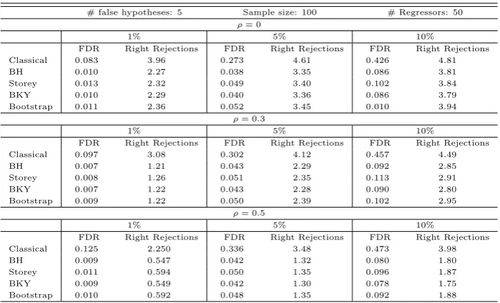
Table 2: Linear regression model with 5 false hypotheses

# false hypotheses: 5 Sample size: 100 # Regressors: 50

ρ= 0

1% 5% 10%

FDR Right Rejections FDR Right Rejections FDR Right Rejections

Classical 0.083 3.96 0.273 4.61 0.426 4.81

BH 0.010 2.27 0.038 3.35 0.086 3.81

Storey 0.013 2.32 0.049 3.40 0.102 3.84

BKY 0.010 2.29 0.040 3.36 0.086 3.79

Bootstrap 0.011 2.36 0.052 3.45 0.010 3.94

ρ= 0.3

1% 5% 10%

Classical 0.097 3.08 0.302 4.12 0.457 4.49

BH 0.007 1.21 0.043 2.29 0.092 2.85

Storey 0.008 1.26 0.051 2.35 0.113 2.91

BKY 0.007 1.22 0.043 2.28 0.090 2.80

Bootstrap 0.009 1.22 0.050 2.39 0.102 2.95

ρ= 0.5

1% 5% 10%

Classical 0.125 2.250 0.336 3.48 0.473 3.98

BH 0.009 0.547 0.042 1.32 0.080 1.80

Storey 0.011 0.594 0.050 1.35 0.096 1.87

BKY 0.009 0.549 0.042 1.30 0.078 1.75

Bootstrap 0.010 0.592 0.048 1.35 0.092 1.88

This table shows the results of a Monte Carlo simulation as specified in section 4.1 with 2000 sim-ulations and the indicated parameter settings. The procedures controlling the FDR were applied as described in section 3. For the Storey procedure,λ= 0.5.

4.1 Linear Regression Model

We simulate a data generating process (DGP) of the following form:

y=Xβ+u.

In the basic setup, X = (x′₁, . . . ,x_k′)′ _{is a} _n_×_k _{matrix of regressors, where each row} _x

i =

(x1i, . . . , xki) is distributed multivariate normal with mean zero, variance one and common

cor-relationρ. The elementsui of the vectoruare iidN(0,1). The vectorβ is k×1. In each setup,

n= 100 andk= 50.5 _{We consider}_ρ₌_{_0,_0.3,_0.5_}_{and investigate three scenarios for the vector}_β_:

• Every tenthβi = 0.5, and the remaining βi = 0, such that there are 5 false hypotheses.6

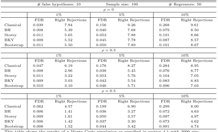
• Every fifthβi = 0.5, and the remainingβi= 0, such that there are 10 false hypotheses.

• Every second βi = 0.5, and the remainingβi= 0, such that there are 25 false hypotheses.

For the case of five false hypotheses, Table 2 shows that all multiple testing procedures control the FDR for any correlation ρ. Classical testing does not; in general FDRs substantially higher than the nominal level of the individual tests result. The violation of the FDR increases in ρ. One reason for this is that the larger ρ, the larger the problem of multicollinearity among the regressors. Hence, the individual t-tests become less reliable. This can also be seen from

5_{Unreported experiments draw qualitatively similar pictures for different}

nandk.

6_{The value 0.5 is chosen so as to be able to discriminate between the rejective power of the procedures. An}

(15)

the fact that the number of right rejections declines for higher ρ. Unsurprisingly, the number of right rejections using classical testing is above that of the multiple testing procedures. But this comes at the price of unacceptable many wrong rejections. Moreover, unlike with multiple testing procedures, the FDR of classical testing is unknown in practice. Hence, the user does not know how many hypotheses are rightfully rejected. Among the FDR controlling procedures the bootstrap yields the highest number of right rejections. This likely is due to the bootstrap method taking the dependence between the test statistics into account. Hence the bootstrap appears to slightly outperform the other FDR controlling procedures.

When either 10 or 25 coefficients are significant, the picture is qualitatively the same.7 Again, all procedures except classical testing control the FDR at the desiredγ. Moreover, the bootstrap approach again appears to be most powerful. The non-control of the FDR using classical testing becomes less severe as the number of false hypotheses increases. In view of the definition of the FDR, E FF₊S

, this should be no surprise. As more variables are rightly declared significant, keeping the total number of false rejections,F, constant, the FDR is lower by construction.

4.2 Pairwise Testing for Output Convergence

As in Pesaran (2007) we use the following DGP

yit=γift+ǫit,

where

ft=ft−1+vt, vt=ρvvt−1+et, et∼iidN(0,1−ρ2v)

and

ǫit=ρiǫi,t−1+νit, νit∼iidN(0, σνi2(1−ρ2i)), σ2νi∼iiduniform[0.5,1.5],

fori= 1,2, . . . , nand t= 1,2, . . . , T. We consider n= 10 and set T = 50 and T = 100.8 When generating the autoregressive processes we start at t=₋49 and discard the first 50 draws. As in Pesaran (2007) we take ρv = 0.6 andρi ∼iiduniform[0.2,0.6]. We only consider one single pool

of convergent countries, i.e. all countries within the pool converge with each other and all others do not. For all converging pairs we setγi =γj = 1. For all others,γi ∼iid χ2κi, whereκi is drawn

with replacement from integers 1 to 10. We consider two scenarios:

• For 3/10 of all countriesγi = 1. Forn= 10 this amounts to 3 convergent pairs.

• For 1/2 of all countriesγi= 1. For n= 10 this amounts to 10 convergent pairs.

7_{Results are available upon request. (Please refer to Tables A.1 and A.2.)}

8_{Due to the large computation time required to find the bootstrap critical values in Algorithm 3.4.4 we only}

(16)

[image:16.595.128.480.112.494.2]

Table 3: Pairwise unit root tests with 10 false hypotheses andT = 50

n= 10[45pairs] T= 50 false hypotheses: 5[10pairs]

OLS detrending GLS detrending

p= 0

FDR Right Rejections FDR Right Rejections

Classical approach 0.203 9.95 Classical approach 0.184 9.94

BH 0.160 9.54 BH 0.142 9.48

Storey 0.281 9.45 Storey 0.179 9.38

BKY 0.171 9.62 BKY 0.150 9.58

Bootstrap 0.168 9.62 Bootstrap 0.154 9.70

p= 1

BH 0.119 7.00 BH 0.115 7.24

Storey 0.316 7.78 Storey 0.284 7.86

BKY 0.126 7.24 BKY 0.123 7.43

p= 3

BH 0.0668 1.85 BH 0.0867 2.26

Storey 0.279 4.63 Storey 0.291 4.82

BKY 0.0648 1.94 BKY 0.0853 2.33

p= 4

BH 0.0505 0.866 BH 0.0636 1.08

Storey 0.272 3.89 Storey 0.266 3.81

BKY 0.0472 0.910 BKY 0.0600 1.13

p= 5

BH 0.0467 0.557 BH 0.0643 0.769

Storey 0.277 3.62 Storey 0.259 3.45

BKY 0.0450 0.637 BKY 0.0630 0.845

p= 10

BH 0.0287 0.0730 BH 0.0498 0.154

Storey 0.190 1.81 Storey 0.162 1.15

BKY 0.0278 0.0840 BKY 0.0469 0.193

This table shows the results of a Monte Carlo simulation as specified in section 4.2 with 1000 sim-ulations and the indicated parameter settings. Tests were conducted forα=γ= 0.05. The FDR controlling procedures applied are described in section 3. For the Storey procedure,λ= 0.5.

(17)

Table 3 shows the results for n= 10, so 45 hypotheses are tested,T = 50 and 10 pairs are signif-icant, i.e. contain no unit root. At any lag length p, classical testing results in a severe violation of the FDR, irrespective of whether OLS or GLS detrending is used. All the other procedures except Storey control the FDR for sufficiently highp.9 A high number of lags is plausible for this DGP, as the dijt are sums of AR(1) processes, that generally follow an ARM A(2,1) (Granger

and Morris, 1976), or AR(_∞), process, that has to be approximated with a high number of lags. Moreover, that FDR control can only be attained for high p is in line with Pesaran (2007), who finds size distortions of the individual tests when p < 4. Given the required p for each FDR controlling procedure, the bootstrap is most powerful. For the BH and the BKY method, GLS detrending yields somewhat higher power than OLS detrending.

VaryingT and the number of false hypotheses leaves the results qualitatively the same.10 _Classical

testing results in a violation of the FDR in all scenarios for OLS as well as GLS detrending. Again, the Storey procedure does not control the FDR. The main difference for T = 100 is that FDR control of the BH, BKY and bootstrap procedure is only attained when p = 6 and p = 12 (corresponding to the rulesp= 6(T /100)1/4 and p= 12(T /100)1/4).

5 Empirical Growth Models Revisited

We now apply the above techniques to two widely used data sets. We first discuss the data, their sources and prior use and then present the results obtained for each. We estimate equation (3) by OLS. Of course, OLS generally produces inconsistent estimators under e.g. endogeneity and/or measurement errors. However, Hauk Jr. and Wacziarg (2009) have recently shown that these and other effects plaguing cross-sectional growth regressions largely cancel out in OLS estimation, making it a superior choice to more complicated estimators like Arellano and Bond’s (1991).

In a third section we compare the results to previous studies that have used these data sets. The first data set is from Fernandez, Ley and Steel (2001) (FLS). It also constitutes the main reference point, since many authors have used this data set to whose results we can compare ours. The second data set was first used in Masanjala and Papageorgiou (2005) (MP).11

5.1 FLS

5.1.1 Data

The FLS data set is a version of that used in Sala-i-Martin (1997). The latter includes n = 140 countries for which GDP growth is computed over the period 1960-1992, and 62 regressors.

9_{We even find that all FDR controlling procedures also control the Familywise Error Rate (FWER), defined as}

the probability of one or more false rejections, a stricter criterion than the FDR.

10_{Results are available upon request. (Please refer to Tables A.3, A.4 and A.5.)}

11_{These data are available at http://econ.queensu.ca/jae/. We also investigated the data set of Sala-i-Martin,}

(18)

[image:18.595.117.492.110.478.2]

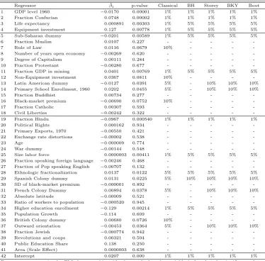
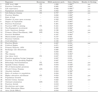
Table 4: Results for the FLS Data Set

Regressor βˆi p-value Classical BH Storey BKY Boot

1 GDP level 1960 −0.0170 0.00001 1% 1% 1% 1% 1%

2 Fraction Confucian 0.0748 0.00002 1% 1% 1% 1% 1%

3 Life expectancy 0.000891 0.00303 1% 5% 5% 5% 5%

4 Equipment investment 0.127 0.00778 1% 5% 5% 5% 5%

5 Sub-Saharan dummy −0.0201 0.00589 1% 5% 5% 5% 5%

6 Fraction Muslim 0.0107 0.227 - - - -

-7 Rule of Law 0.0116 0.0679 10% - - -

-8 Number of years open economy −0.00269 0.620 - - - -

-9 Degree of Capitalism 0.00111 0.284 - - - -

-10 Fraction Protestant −0.00280 0.677 - - - -

-11 Fraction GDP in mining 0.0401 0.00769 1% 5% 5% 5% 5%

12 Non-Equipment investment 0.0367 0.0811 10% - - -

-13 Latin American dummy −0.0127 0.0391 5% - 10% 10% 10%

14 Primary School Enrollment, 1960 0.0202 0.0455 5% - 10% 10% 10%

15 Fraction Buddhist 0.00734 0.277 - - - -

-16 Black-market premium −0.00690 0.0752 10% - - -

-17 Fraction Catholic 0.00307 0.593 - - - -

-18 Civil Liberties −0.00242 0.322 - - - -

-19 Fraction Hindu −0.0967 0.000540 1% 1% 1% 1% 1%

20 Political Rights 0.000162 0.934 - - - -

-21 Primary Exports, 1970 −0.00550 0.421 - - - -

-22 Exchange rate distortions −0.00002 0.538 - - - -

-23 Age −0.000009 0.774 - - - -

-24 War dummy −0.00144 0.548 - - - -

-25 Size labor force 0.0000003 0.00411 1% 5% 5% 5% 5%

26 Fraction speaking foreign language −0.00246 0.468 - - - -

-27 Fraction of Pop speaking English −0.00707 0.132 - - - -

-28 Ethnologic fractionalization 0.0137 0.0122 5% 5% 5% 5% 5%

29 Spanish Colony dummy 0.0131 0.0225 5% 10% 10% 10% 10%

30 SD of black-market premium −0.000001 0.892 - - - -

-31 French Colony Dummy 0.00894 0.0378 5% - 10% 10% 10%

32 Absolute latitude −0.00009 0.521 - - - -

-33 Ratio of workers to population −0.000520 0.945 - - - -

-34 Higher education enrollment −0.129 0.00214 1% 5% 5% 5% 5%

35 Population Growth −0.114 0.609 - - - -

-36 British Colony dummy 0.00680 0.0726 10% - - -

-37 Outward orientation −0.00453 0.0364 5% - 10% 10% 10%

38 Fraction Jewish −0.000774 0.942 - - - -

-39 Revolutions and coups 0.00321 0.504 - - - -

-40 Public Education Share 0.138 0.250 - - - -

-41 Area (Scale Effect) 0.0000003 0.638 - - - -

-42 Intercept 0.0207 0.000 1% 1% 1% 1% 1%

For every regressor in the FLS data set this table shows whether the variable is found to be significant when controlling the FDR at the indicated level. The procedures are described in section 3. We work with 5000 bootstrap iterations. In the Storey approachλ= 0.5.

Fernandez et al. (2001) only include those countries for which observations on all 25 variables flagged important by Sala-i-Martin (1997) are available. This amounts to n = 72. They then add all variables which do not induce any missing observations in these countries. This yields 41 variables. Using this data set allows us to compare our findings to those of Fernandez et al.

(2001), Sala-i-Martin (1997), Hendry and Krolzig (2004) and Ley and Steel (2009).

5.1.2 Results

(19)

[image:19.595.147.455.97.307.2]

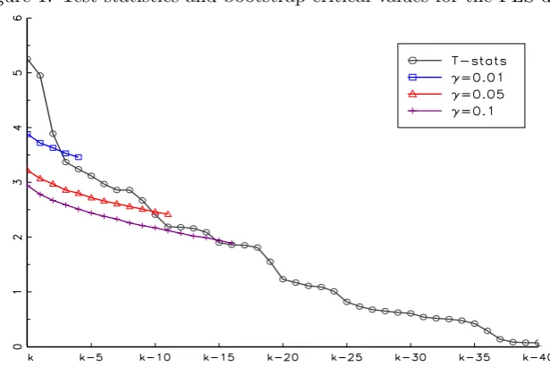
Figure 1: Test statistics and bootstrap critical values for the FLS data

The test statistics Ti and the relevant bootstrap critical values ˆcγ,j (i.e. those until and around Ti < cˆγ,i) for differentγplotted againstk, the ranks of theTi.

using HC2 are similar to the OLS results; using HC3 resulted in substantially fewer rejections.12

Classical testing declares 20 variables (excluding the intercept) to be significant at the 10% level, 15 at the 5% level and 9 at the 1% significance level. The picture is different when accounting for multiple testing by controlling the FDR. The most rejective and still reliable procedure according to the Monte Carlo study, the bootstrap method, declares 15 variables significant at γ = 0.1, 10 at γ = 0.05 and when controlling the FDR at the 1% level, only 3 variables are found to be significantly related to GDP growth. (See Figure 1 for a graphical illustration.) We will elaborate on the three variables later. Hence, this simple comparison reveals that several variables appear to be only spuriously declared significant because of the large number of hypothesis tests performed. Unreported additional simulations13 as in section 4 with 10 (out of 50) false hypotheses find an FDR of classical testing of around 1/3. To the extent that the MC study of sec. 4 is representative for the present empirical application, we should therefore expect roughly 1 false for every 3 rejections when testing atα= 0.1. This would mean that we should expect around 14(= 20₋6) of the 20 rejections to be correct. This is in line with the bootstrap results, where around (1₋0.1)_×15_≈13₋14 of the rejections can be expected to be correct. Of course, such corrective reasoning for classical testing hinges on Monte Carlo designs that may or may not yield estimated FDRs representative for the empirical study under consideration. A key advantage of multiple testing techniques is that FDR control obtains under much more general conditions, as evidenced

12_{Performing a White type test for heteroscedasticity would be pointless here, since the null of no}

heteroscedas-ticity would never be rejected because of the high number of variables included in the model. The 95% critical value of the 800 degrees of freedom test is 866.9, whereasn·R2 of the test regression is bounded above by 72. (Please

refer to Tables A.7 and A.8.)

(20)

[image:20.595.112.498.112.470.2]

Table 5: Comparison FLS Data Set

Regressor Bootstrap BMA posterior prob. Sala-i-Martin Hendry & Krolzig

1 GDP level 1960 1% 1.000 1.000∗∗ _yes

2 Fraction Confucian 1% 0.995 1.000∗ _yes

3 Life expectancy 5% 0.946 0.999∗∗ _yes

4 Equipment investment 5% 0.942 1.000∗ _yes

5 Sub-Saharan dummy 5% 0.757 0.997∗ _yes

6 Fraction Muslim - 0.656 1.000∗

-7 Rule of Law - 0.516 1.000∗

-8 Number of years open economy - 0.502 1.000∗ _yes

9 Degree of Capitalism - 0.471 0.987∗

-10 Fraction Protestant - 0.461 0.966∗

-11 Fraction GDP in mining 5% 0.441 0.994∗ _yes

12 Non-Equipment investment - 0.431 0.982∗

-13 Latin American dummy 10% 0.190 0.998∗ _yes

14 Primary School Enrollment, 1960 10% 0.184 0.992∗∗ _yes

15 Fraction Buddhist - 0.167 0.964∗

-16 Black-market premium - 0.157 0.825

-17 Fraction Catholic - 0.110 0.963∗

-18 Civil Liberties - 0.100 0.997∗

-19 Fraction Hindu 1% 0.097 0.654 yes

20 Political Rights - 0.071 0.990∗

-21 Primary Exports, 1970 - 0.069 0.998∗

-22 Exchange rate distortions - 0.060 0.968∗

-23 Age - 0.058 0.903

-24 War dummy - 0.052 0.984∗

-25 Size labor force 5% 0.047 0.835 yes

26 Fraction speaking foreign language - 0.047 0.831

-27 Fraction of Pop speaking English - 0.047 0.910∗

-28 Ethnologic fractionalization 5% 0.035 0.643 yes

29 Spanish Colony dummy 10% 0.034 0.938∗ _yes

30 SD of black-market premium - 0.031 0.993∗

-31 French Colony Dummy 10% 0.031 0.702 yes

32 Absolute latitude - 0.024 0.980∗

-33 Ratio of workers to population - 0.024 0.766

-34 Higher education enrollment 5% 0.024 0.579 yes

35 Population Growth - 0.022 0.807

-36 British Colony dummy - 0.022 0.579 yes

37 Outward orientation 10% 0.021 0.634

-38 Fraction Jewish - 0.019 0.747

-39 Revolutions and coups - 0.017 0.995∗

-40 Public Education Share - 0.016 0.580

-41 Area (Scale Effect) - 0.016 0.532

-“Bootstrap” denotes significance when controlling the FDR at the indicated level; “BMA post. prob.” denotes the marginal posterior probability of inclusion found in Fernandezet al.(2001); “Sala-i-Martin” shows the CDF(0), explained in section 5.1.3, found in Sala-i-Martin (1997), where∗∗indicate variables always included and∗indicate variables found significantly related to growth; “Hendry and Krolzig” shows a “yes” if the variable is included following the procedure in Hendry and Krolzig (2004).

by our and many other studies and theoretical contributions.

(21)

5.1.3 Comparison to Previous Studies

Fernandez et al. ₍₂₀₀₁₎ _{Table 5 compares our findings to those of Fernandez} _{et al.} _(2001).

To be able to better compare the findings, we briefly explain the concept of marginal inclusion probability, which is key in Fernandez et al. (2001) to judge the importance of a variable in a regression.

Fernandez et al.(2001) use BMA techniques to account for the model uncertainty in the growth regression context. Given the 41 possible explanatory variables there are 241 possible correct models, assuming that these nest the true DGP. One now has to assign a ‘prior distribution’ to each model as well as to the inclusion of a certain variable in each model. We will elaborate on the influence of these choices in section 5.1.3. Using Bayes’ law Fernandezet al.(2001) then compute the ‘posterior inclusion probability’ of each of the 241 _{possible models: “The marginal posterior}

probability of including a certain variable is simply the sum of the posterior probabilities of all models that contain this regressor.” The Bayesian framework provides no cut-off value for the marginal inclusion probability of a variable to declare it (non-)significant. Nevertheless, one gets a good feeling of the importance of each variable.

Table 5 shows that the five variables with the highest marginal posterior probability of inclusion in Fernandez et al. (2001) are also significant according to the bootstrap method at γ = 0.05. But there are also variables which are significantly related to growth using our approach which have a marginal posterior probability below 0.1. For example, “Fraction Hindu” is significant at γ = 0.05 while its marginal posterior probability is only 0.097. Hence, there are non-negligible differences between the two approaches.

Sala-i-Martin (1997) We now compare the results of the FLS data set with those of Sala-i-Martin (1997). His approach is as follows: In every regression run, there are three sets of variables,

w, v and q. w consists of the three variables, namely “GDP level in 1960”, “Life expectancy” and “Primary school enrolment”. These three variables are included in every regression. v is the variable under study and q is a trio of the other remaining 58 variables. He then computes the cumulative distribution function (CDF) of the coefficient corresponding tovat zero by averaging the coefficient of v obtained in the regressions for all combinations of variables in q.14 Since a variable can have a positive or negative coefficient he sets CDF(0) = max_{CDF(0),1₋CDF(0)_}. He then flags a variable significantly related to growth if its CDF(0)_≤0.91. The outcome of this approach depends on a large set of misspecified regressions, in particular via the omitted variable bias inherent when conducting many overly short regressions.

Sala-i-Martin (1997) finds the same five variables to be significant that were already significant in both the bootstrap approach and in Fernandezet al. (2001) (Table 5). But beyond that, there seems to be little agreement concerning significance of variables in Sala-i-Martin (1997) and in our

14_{This results in 455,126 different models. The two million regressions in his title arise because any model is}

(22)

study. Out of the 25 variables15 flagged significant by Sala-i-Martin (1997), we can only confirm 9 using an FDR up to 10%.

Hendry and Krolzig (2004) Hendry and Krolzig (2004) also use the FLS data. They argue that if the general unrestricted model (GUM) provided by all available explanatory variables nests a good approximation of the DGP, then a “General to simple” (Gets) selection based approach would suffice to find the best model. Of course, this abstracts from problems like data accuracy, exogeneity of regressors or constancy of the parameters across observations. But this abstraction is inherent to all approaches presented here, including the one we propose. Hendry and Krolzig (2004) further note that if all regressors were mutually orthogonal, then selection based on the ordered squared t-statistics from the GUM, say t2

(1) ≥ t2(2) ≥ . . . ≥ t2(k), could be validly used

for model selection. One would then declare variables 1, . . . ,k˜ with t2

(˜k)≥cα significant and the

remaining ones insignificant, where t2

(˜k+1) ≤cα. They choose α = 0.025 so as to only select one

variable by chance out of thek= 41 regressors. Sincet-values in fact are not mutually orthogonal, a multi-path search introduced in Hoover and Perez (1999) is used. This approach is somewhat similar to the one employed here, where decisions are also based on individual t-statistics and their dependence is taken into account using the bootstrap approach described in section 3.3. The bootstrap approach may be more transparent for the user—all one has to choose is someγ. Transparent cutoffs ˆcj are then provided, and no multi-path search is needed.

The similarity of the two approaches can be seen when comparing the variables found significant (Table 5). The number of significant variables in Hendry and Krolzig (2004) is 16 compared to 15 for our approach, out of which 14 coincide. (A J-test rejects both models, although Hendry and Krolzig’s model is rejected only at larger significance values.) Again, the five variables already jointly significant in Fernandezet al.(2001) and Sala-i-Martin (1997) are also significant in Hendry and Krolzig (2004). Hence, we are quite confident regarding the importance of “GDP level 1960”, “Fraction Confucian”, “Life expectancy”, “Equipment investment” and “Sub-Saharan dummy”.

Ley and Steel (2009) Results from BMA techniques to account for model uncertainty in growth regression are potentially sensitive to choices made by the modeler. This problem is identified among others in Ley and Steel (2009). They consider BMA on linear regression models Mj with 0≤kj ≤k regressors grouped inXj leading to

y_|a,βj, σ∼N(aι+Xjβj, σ2I),

whereβj ∈Rkj and σ∈R+ is a scale parameter.

One then needs to specify the prior distribution of each parameter for model Mj as well as the

prior distribution of the inclusion of modelMj. For the prior density of the parameters, Ley and

Steel (2009) use a combination of a so called ‘non-informative’ improper priors on a and σ as well as a ‘g-prior’ on β. Ley and Steel (2009) advocate choosing g = 1/maxn, k2 . The prior

(23)

model probabilities are often specified as P(Mj) =θkj(1−θ)k−kj, assuming that each regressor

enters a model with equal probability and independently of the others. Fernandez et al. (2001) choose θ= 0.5, implying an expected model size of m=k/2. Ley and Steel (2009) also consider choosingθrandomly. In that case, one first fixes the expected model size mand then determines the interval in whichθ can vary.

Ley and Steel (2009) show that when using the above priors in the FLS data set, the posterior mean model size ranges from 6.03 with m = k/2 = 20.5, random θ and g = 1/k2 _{to 19.84}

for m = k/2 = 20.5, fixed θ and g = 1/n. Their Table II shows the ranking of the marginal posterior probability of including a certain variable to also be highly sensitive to the prior settings. Comparing cases withg= 1/nand fixedθthey note: “Fraction Hindu, the Labor force size, and Higher education enrolment go from virtually always included with m = 20.5 to virtually never included with m= 7.”

These findings might help explain the differences between the bootstrap approach and the marginal posterior inclusion probabilities found in Fernandez et al. (2001). Moreover, it might also be a reason for the differences between the latter and the variable selection in Sala-i-Martin (1997). In general the findings in Ley and Steel (2009) cast doubt on the robustness of BMA techniques. A more transparent and robust selection of variables is obtained using e.g. the FDR controlling bootstrap approach presented here.

5.2 MP Data Set

5.2.1 Data

The data set covers 93 countries, for which average GDP growth was calculated from 1960 to 1992. It was developed and first used in Masanjala and Papageorgiou (2005). The data set consists of 32 basic variables out of which 22 are also combined with an interaction dummy for African countries. Thus,k = 54 here. To tackle the endogeneity issues Masanjala and Papageorgiou (2005) devote careful attention to only including predetermined variables. Furthermore, the interaction dummies address possible parameter heterogeneity.

5.2.2 Results

Table 6 shows the results when accounting for multiple testing by controlling the FDR in the MP data set.16 _{Only three variables are found to be significantly related to GDP growth, namely}

“ln GDP per capita, 1960” (at γ = 0.05), “Life expectancy”(at γ = 0.01) and “A_∗Mining”(at γ = 0.01) using the bootstrap method.17 Again the difference to the number of significant variables using classical testing is substantial. Classical testing finds 13 significant variables at

16_{We also calculate robust standard errors. The results are qualitatively the same as for the FLS data set.} 17_{For the MP data set, the BH method and the BKY algorithm yield the same results; the Storey method finds}

(24)

[image:24.595.117.493.109.548.2]

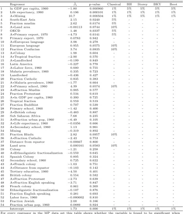
Table 6: MP Data Set

Regressor βˆi p-value Classical BH Storey BKY Boot

1 ln GDP per capita, 1960 −1.80 0.000960 1% 5% 5% 5% 5%

2 Life expectancy, 1960 0.196 0.000101 1% 1% 1% 1% 1%

3 A∗Mining 10.7 0.000504 1% 1% 5% 1% 1%

4 South-East Asia 2.15 0.0240 5% - - -

-5 Fraction muslim 2.62 0.0174 5% - - -

-6 A∗Land area −0.00113 0.0744 10% - - -

-7 OECD 1.48 0.0337 5% - - -

-8 A∗Primary export, 1970 −4.73 0.0141 5% - - -

-9 Primary export, 1970 0.0783 0.942 - - - -

-10 A∗European language 3.98 0.278 - - - -

-11 European language 0.955 0.0575 10% - - -

-12 Fraction Confucian 3.74 0.0835 10% - - -

-13 A∗Colony 1.98 0.604 - - - -

-14 A∗Tropical fraction −2.90 0.570 - - - -

-15 A∗Landlocked −0.199 0.849 - - - -

-16 Latin America −0.227 0.778 - - - -

-17 A∗Labor force, 1960 0.000 0.755 - - - -

-18 Malaria prevalence, 1960 0.335 0.723 - - - -

-19 Landlocked −0.436 0.427 - - - -

-20 Fraction Catholic 0.835 0.383 - - - -

-21 A∗Malaria prevalence, 1960 −1.77 0.664 - - - -

-22 A∗Primary school, 1960 4.39 0.0574 10% - - -

-23 A∗Fraction Muslim 0.905 0.577 - - - -

-24 Fraction Protestant 0.534 0.619 - - - -

-25 A∗ln GDP per capita, 1960 0.300 0.725 - - - -

-26 Tropical fraction 0.559 0.519 - - - -

-27 Fraction Buddhist 0.707 0.539 - - - -

-28 Primary school, 1960 −1.42 0.400 - - - -

-29 A∗British colony −0.483 0.887 - - - -

-30 Sub Saharan Africa 7.68 0.235 - - - -

-31 A∗Fraction urban pop, 1960 −6.49 0.105 - - - -

-32 A∗Life expectancy, 1960 −0.0356 0.666 - - - -

-33 A∗Secondary school, 1960 1.13 0.961 - - - -

-34 Mining −0.319 0.892 - - - -

-35 Fraction Hindu 2.82 0.0957 10% - - -

-36 A∗Fraction Catholic −2.43 0.753 - - - -

-37 Distance from equator −0.00667 0.800 - - - -

-38 Land area 0.000161 0.0583 10% - - -

-39 Colony −1.21 0.258 - - - -

-40 A∗Ethnoliguistic fractionalization −0.559 0.645 - - - -

-41 Spanish Colony 0.895 0.324 - - - -

-42 Secondary school, 1960 0.725 0.622 - - - -

-43 A∗French colony −1.03 0.751 - - - -

-44 A∗Distance from equator −0.103 0.142 - - - -

-45 Tertiary education, 1960 −4.50 0.401 - - - -

-46 British colony 0.554 0.582 - - - -

-47 A∗Fraction Protestant −2.73 0.639 - - - -

-48 A∗Fraction English speaking −3.71 0.847 - - - -

-49 French colony 0.861 0.369 - - - -

-50 Ethnoliguistic fractionalization −0.107 0.876 - - - -

-51 Fraction English speaking 0.281 0.693 - - - -

-52 Labor force, 1960 −0.000002 0.810 - - - -

-53 Fraction Jewish 2.00 0.166 - - - -

-54 Fraction urban pop, 1960 0.0889 0.924 - - - -

-Intercept 1.73 0.000 1% 1% 1% 1% 1%

For every regressor in the MP data set this table shows whether the variable is found to be significant when controlling the FDR at the indicated level. The procedures are described in section 3. We work with 5000 bootstrap iterations. In the Storey approachλ= 0.5.

α= 0.1. Compared to the FLS data, a possible reason for the larger difference between classical testing and FDR controlling testing is the larger number of explanatory variables. This results in stricter FDR controlling tests. (Of course, it is also simply other data.)

5.2.3 Comparison to Previous Studies

(25)

[image:25.595.188.416.109.225.2]

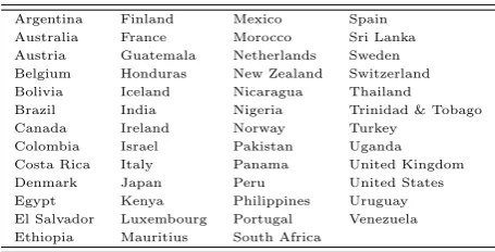
Table 7: Countries Included

Argentina Finland Mexico Spain

Australia France Morocco Sri Lanka

Austria Guatemala Netherlands Sweden Belgium Honduras New Zealand Switzerland

Bolivia Iceland Nicaragua Thailand

Brazil India Nigeria Trinidad & Tobago

Canada Ireland Norway Turkey

Colombia Israel Pakistan Uganda

Costa Rica Italy Panama United Kingdom

Denmark Japan Peru United States

Egypt Kenya Philippines Uruguay

El Salvador Luxembourg Portugal Venezuela Ethiopia Mauritius South Africa

confirm two. On the other hand, “A*Mining” only has marginal posterior probability of 76.1, yet it is found significant by the FDR controlling techniques. Hence, again the BMA results differ somewhat from the multiple testing results.18 Ley and Steel (2009) also use this data set to investigate the influence of the priors on the outcome of BMA. Again, depending on the different choices, the average posterior model size ranges from 5.42 (m= 7, randomθ, g= 1/k2) to 17.90 (m= 27, fixedθ, g= 1/n). Thus, BMA results are again sensitive to the modeler’s choices.

6 Output Convergence Revisited

We now employ the FDR controlling techniques described in section 3 to a data set of n = 51 countries ranging from 1950 to 2003, so T = 54. The resulting number of different country pairs is 1275. The data is from the Penn World Tables Version 6.2 (Heston, Summers and Aten, 2006) and includes all countries for which data on per-capita output was available for the indicated time span.19 _{We employ standard ADF tests and ADF-GLS tests. The deterministic}

component also includes a time trend. We choose the lag lengthp according to p = 5(T /100)1/4 andp= 6(T /100)1/4 as those yielded the highest number of right rejections while still controlling the FDR for the bootstrap procedure whenT = 50, which is close to the actualT. For the present data this results inp= 4 and p= 5. Critical values andp-values are adjusted to sample size.

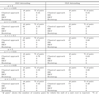
Table 4.2 shows the results of applying the FDR controlling techniques to testing for pairwise convergence. We corroborate the results of Pesaran (2007) that the null of no convergence is only rejected for a fraction of countries less than or equal to the individual significance level of the unit root test applied. When accounting for the multiplicity of tests performed, for no level γ do we find any rejection of the null; this also holds in particular for the most powerful FDR controlling procedure, the bootstrap method using either OLS or GLS detrending.20

18_{For a comparison of the marginal posterior probability to our results refer to Table A.9.} 19_{Table 7 gives a complete list of countries included in the analysis.}

20_{As Pesaran (2007), we also perform analogous exercises for subgroups like European or American countries.}

(26)

[image:26.595.134.471.109.427.2]

Table 8: Pairwise Test for Output convergence

OLS detrending GLS detrending

p= 4

α=γ= 0.01

# pairs % of pairs # pairs % of pairs

Classical approach 2 0.16 Classical approach 3 0.24

BH 0 0 BH 0 0

BKY 0 0 BKY 0 0

Bootstrap 0 0 Bootstrap 0 0

α=γ= 0.05

BH 0 0 BH 0 0

BKY 0 0 BKY 0 0

α=γ= 0.1

BH 0 0 BH 0 0

BKY 0 0 BKY 0 0

p= 5

α=γ= 0.01

BH 0 0 BH 0 0

BKY 0 0 BKY 0 0

α=γ= 0.05

BH 0 0 BH 0 0

BKY 0 0 BKY 0 0

α=γ= 0.1

BH 0 0 BH 0 0

BKY 0 0 BKY 0 0

“# pairs” shows the number of country pairs for which the null of a unit root is rejected. “% of pairs” shows the proportion of those pairs compared to the total number of pairs. The procedures are described in section 3. We use 5000 bootstrap iterations. In the Storey approach,λ= 0.5.

At first glance, this finding might seem a bit surprising. But this finding clarifies the results in Pesaran (2007).21 His approach does not allow to say whether rejection of the null for some country pairs was spurious or not. Finding no converging pairs when employing a more appropriate testing framework for individual tests (rather than for fractions of rejections), the confidence in Pesaran’s no time-series convergence finding is strengthened.

Nevertheless, we emphasize that cross-country convergence was tested using a very strict defini-tion (Islam, 2003). We cannot rule out cross-country convergence using for example condidefini-tional definitions nor do we make any statements about ‘within convergence’ here, i.e. whether countries converge to a steady state output. Indeed we found evidence for ‘within convergence’ in section 5 as initial GDP was always included in the final model. Hence, we do not claim that there is no convergence of economies, but that convergence across economies using a time series definition with the necessary condition of no unit root in the log per-capita output gap of two economies does not appear to hold.

21_{As we have shown in the Monte Carlo study, we also control the FWER at}

(27)

7 Conclusion

This paper highlights the importance of accounting for the multiplicity of tests performed in two applications to growth econometrics. Controlling the FDR, we have shown how to robustly select explanatory variables in cross-sectional growth regressions. Among others, this was done using a bootstrap approach which takes the dependence structure of the test statistics into account and thus has high power. The outcome of other approaches in cross-sectional growth regressions, such as Bayesian Model Averaging, is sensitive to user choices and hence may not be robust. In addition to the robustness of our bootstrap approach, we believe the selection of variables using FDR controlling techniques to be very transparent for the user. The only choice to make is the level at which one wants to control the FDR.

The actual variables selected support the neoclassical growth theory and its implied convergence of countries to a steady state output. The second application investigates cross-country conver-gence using pairwise unit-root tests. Controlling the FDR, we find no evidence of this type of convergence. This clarifies the results of Pesaran (2007), whose framework does not allow to say whether the fraction of rejected pairs is spurious or not.

There are more fields in econometrics where accounting for multiplicity is important. For exam-ple, modeling returns to schooling involves a large number of candidate explanatory variables. As we have shown in the application to cross-sectional growth regressions, classical significance tests produce a non-negligible number of variables which appear to be only spuriously significant because of the large number of tests performed. As such, the techniques studied here may prove fruitful in many other literatures.

References

Arellano M, Bond S. 1991. Some tests of specification for panel data: Monte Carlo evidence and an application to employment equations.Review of Economic Studies 58: 277–297.

Barro RJ. 1991. Economic growth in a cross section of countries.The Quarterly Journal of Economics106: 407–443. Barro RJ, Sala-i-Martin XX. 1995.Economic Growth. McGraw Hill.

Benjamini Y, Hochberg Y. 1995. Controlling the false discovery rate: A practical and powerful approach to multiple testing.Journal of the Royal Statistical Society. Series B57: 289–300.

Benjamini Y, Krieger AM, Yekutieli D. 2006. Adaptive linear step-up procedure that control the false discovery rate.Biometrika93: 491–507.

Benjamini Y, Yekutieli D. 2001. The control of the false discovery rate in multiple testing under dependency.The Annals of Statistics 29: 1165–1188.

Bernard A, Durlauf S. 1995. Convergence in international output.Journal of Applied Econometrics 10: 97–108. Burridge P, Taylor AMR. 2004. Bootstrapping the HEGY seasonal unit root tests.Journal of Econometrics 123:

67–87.

Campbell Y, Mankiw N. 1989. International evidence on the persistence of economic fluctuations.Journal of

Mon-etary Economics 23: 319–333.

Demetrescu M, Hassler U, Kuzin V. 2008. Pitfalls of post-model-selection testing: Experimental quantification.