Probabilistic QOS Aware Congestion Control in Wireless Multimedia Sensor Networks

http://dx.doi.org/10.4236/cs.2016.79181

How to cite this paper: Mayandi, M. and Pillai, K.V. (2016) Probabilistic QOS Aware Congestion Control in Wireless Multi-media Sensor Networks. Circuits and Systems, 7, 2081-2094. http://dx.doi.org/10.4236/cs.2016.79181

Probabilistic QOS Aware Congestion Control

in Wireless Multimedia Sensor Networks

Muthuselvi Mayandi1*_{,Kavitha Velayudhan Pillai}2

1_{Department of Computer Science and Engineering, University College of Engineering Nagercoil,}

Anna University, Chennai, India

2_{Department of Computer Science and Engineering, University College of Engineering Kancheepuram,}

Anna University, Chennai, India

Received 30 April 2016; accepted 25 May 2016; published 5 July 2016

Copyright © 2016 by authors and Scientific Research Publishing Inc.

This work is licensed under the Creative Commons Attribution International License (CC BY).

http://creativecommons.org/licenses/by/4.0/

Abstract

The general problem faced in the field of Wireless Multimedia Sensor Networks (WMSNs) is con-gestion. The most common method in the area of WMSNs to minimize congestion is traffic control. Quality Of Service (QOS) is widely used in WMSNs to guarantee preferential service for critical ap-plications by controlling end-to-end delay, reducing data loss and by providing adequate band-width. The present work is on Probabilistic QOS Aware Congestion Control (PQACC) which em-ploys probabilistic method based congestion prediction and priority based data transmission rate adjustment, where inelastic real-time traffic and elastic non-real-time traffic are treated sepa-rately. Using the present PQACC approach, average throughput, average source-to-sink delay and average packet loss probability are improved by 9%, 10.33% and 16.03% compared to EWPBRC and achieved 5.97%, 7.05% and 11.69% improvement compared to FEWPBRC. Simulation result reveals that, congestion is effectively predicted, controlled andprovides necessary level of QOS in terms of delay, throughput and packet loss, hence making this approach possible in mission criti-cal applications.

Keywords

Congestion Control, WMSN, Traffic Control, QOS, Probabilistic Method, Inelastic Traffic, Elastic Traffic

1. Introduction

Recent advances and development in the field of sensors and availability of economical hardware such as

crophone and Complementary Metal Oxide Semiconductor (CMOS) camera allow the emerging of WMSNs. Wireless multimedia sensor network is a collection of a huge number of wireless sensors outfitted with devices which are capable of sensing and retrieving images, audio/video streams and scalar data [1]. And the importance of the traffic generated by these sensors is different; it is needed that preference must be given to packets carry-ing important data by providcarry-ing more network resources than other packets to achieve diverse levels of service

[2]. To provide different levels of service to traffic flows with different service requirements in terms of delay, throughput and packet loss, a priority can be assigned to each different traffic flow. The two kinds of data traffic supported by WMSNs are InElastic Real Time (IERT) and Elastic Non Real Time traffic (ENRT). ENRT can adapt to extensive changes in throughput and delay while IERT does not adjust with changes in throughput and delay. Hence IERT necessitates preferential treatment [3]. The major applications of WMSNs include multime-dia surveillance, traffic control, health care, object locating system and process control in industries [4].

WMSNs face problems due to resource-constrained nature of sensor nodes such as limited energy, processing capacity, bandwidth and small memory. In WMSNs applications, the tiny size of sensors, consumption of power due to heavy volume of traffic and complex computations lead to congestion which subsequently diminishes QOS of applications. Hence the main objective of WMSNs is to develop algorithms that prolong the lifetime of the network and alsoassuresto provide QOS necessities insisted by the applications [5].

The present study is based on the following considerations: a probability based congestion prediction; a mix-ture of three parameters to attain accurate determination of congestion; service discrimination among different kinds of data; an algorithm for rate adjustment based on probability based congestion prediction, priority of the source data and location of source sensors.

2. Related Work

Congestion in WSN may occur because of two reasons [6]: collision in the medium or overflow in the buffer. This will result in retransmissions and dropping of packets which leads to long delay, energy waste, high re-sponse time and low throughput. In WMSN to reduce the effect of congestion, an efficient method is needed to control congestion. Any congestion control technique involves 3 steps [7]: detection of congestion, notification about congestion and adjustment in data rate. In WMSN congestion can be alleviated either end-to-end or hop- by-hop. The hop-by-hop approach is better compared to end-to-end approach due to lower time and energy consumption. Various parameters that are useful for detecting congestion are: buffer occupancy, channel load, packet service time, packet inter arrival time and mixing of the above parameters [8]. The occurrence of conges-tion can be propagated to the rest of the nodes in the network either using implicit method [9] or in explicit way

[10]. In the first method control packets carrying current state of congestion are propagated by congested nodes to other nodes in the network using broadcast nature of WSN. These additional packets will increase the net-work load further which leads to more congestion. In implicit method information about congestion is propa-gated to other nodes in the network using header portion of a data packet or using ACK packets with the help of piggybacking concept. This method does not add any additional load to the network. Congestion can be alle-viated either by controlling the load known as traffic control [9] or by increasing the availability of resources known as resource control [6] otherwise, holes will be created in the network due to power exhaustion of nodes in the congested area. Compared to resource control method, traffic control method will effectively save the re-sources by adjusting the data rate of source node(s) and/or intermediate node(s) in the congested area.

suggested three mechanisms to alleviate congestion. In the first mechanism hop-by-hop flow control, each child node stops its forward transmission once it overhears a packet with congestion indication from its parent. In case of persistent congestion backpressure message will reach the source and it is forced to adjust its rate. The second mechanism namely source limiting uses token bucket algorithm to regulate the traffic. The third mechanism pri-oritized MAC gives preference to nodes that experience congestion than non-congested nodes using randomized back off algorithm. Interference aware Fair Rate Control (IFRC) algorithm [15] uses average buffer occupancy as a parameter for detecting congestion and it controls congestion by altering the outgoing rate of each link us-ing AIMD scheme. In Sink-to-Sensors Congestion Control (CONSISE) approach [16] each upstream node de-tects the current level of congestion based on the outgoing rate of its downstream nodes. Each downstream node is allowed to choose a suitable upstream node to forward packets. At the time of congestion, the unselected up-stream nodes will reduce their outgoing rate.

CODA [11], Fusion [14] and IFRC [15] use a static threshold value for detecting the inception of congestion. But finding such a static value in a dynamic environment is a complicated process. CODA [11] and Fusion [14]

use the broadcast nature of WMSN to give feedback about congestion to neighboring nodes even though there is no guarantee for broadcasted messages. PCCP [12] [13], EWPBRC [3] and FEWPBRC [1] ignore buffer occu-pancy in detecting the inception of congestion that results in repeated buffer overflow. CCF [9] provides only equal fairness among nodes. But in applications where diverse sensors are deployed in different geographical locations purposely, to get dissimilar throughput dependent on priority, CCF cannot be used.

The literature review shows that the probability based approach that considers a combination of buffer occu-pancy, incoming and outgoing data rates for congestion prediction is not proposed so far, by any priority aware congestion control protocol. The present work uses a dynamic threshold value for predicting congestion com-pared to other existing works. It considers buffer occupancy as one of the parameter to predict congestion. It uses piggybacking concept to propagate feedback about congestion that assures guaranteed delivery of packets.

3. Probabilistic QOS Aware Congestion Control Approach

The present work is motivated from the limitations of EWPBRC [3] and Probability approach [17] [18]. EWPBRC [3] detects congestion using input and output data rate alone. Since usage of buffer is not included as a parameter for detecting congestion, overflow of buffer happens frequently that leads to packet loss, throughput minimization and long delay in delivering data. Probability approach [17] [18] makes equal rate adjustment for all the nodes including the source nodes. However in WMSN, sensor nodes may be deployed in various geo-graphical locations based on their importance and hence they need service differentiation.

[image:3.595.143.488.602.707.2]

In the present work, a probability based approach that considers three parameters namely buffer occupancy, incoming and outgoing data rates is used for detecting congestion intensity. Moreover during rate adjustment, preferential treatment is given to sensor nodes based on the class of data generated and their geographical loca-tions.

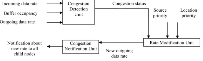
Figure 1 shows the structure of proposed congestion control unit. Similar to other congestion control ap-proaches, this structure in each sensor node includes Congestion Detection Unit (CDU), Rate Modification Unit (RMU) and Congestion Notification Unit (CNU).

CDU unit is used to predict congestion in each sensor node. In the present work, CDU unit computes incom-ing and outgoincom-ing data rate and buffer occupancy of each sensor node to assess the congestion status usincom-ing prob-abilistic method. The value of congestion status may be a negative or positive number. In each predetermined periodic time interval, the outgoing data rate of the children nodes is computed by each parent node in addition

to its own traffic. The priority of sensor nodes differ from one another since these may be fitted with a variety of sensors. Hence each parent node must consider the priority of its children in determining the outgoing data rate of the child nodes. In WMSN, sometimes sensor nodes are purposely deployed in different geographical loca-tions based on their importance, so that sensor nodes may have dissimilar priorities. RAU unit determines the new outgoing data rate by considering the current congestion status, priority of source data and priority based on location of sensor node. The new outgoing data rate is forwarded to CNU unit to notify about the new rate to child nodes. For efficient utilization of network energy, in the present work, CNU unit uses implicit method for communicating notification about congestion. Upon receiving congestion notification each sensor node adjusts its current outgoing data rate according to the value of congestion status.

3.1. Probabilistic Congestion Prediction Approach (PCPA)

The PCPA predicts the congestion intensity in each sensor node with probabilistic approach using dynamic threshold index value on buffer capacity and buffer occupancy of that node. The value of threshold index varies from time to time based on incoming and outgoing data rates of sensor node and remaining space in the buffer.

At time “t + 1”for node “i”, buffer occupancy,

(

1

)

( )

( )

( )

i i i i

b t+ =b t +g t −h t (1)

where g t_i

( )

and h t_i

( )

are the incoming and outgoing data rates for node “i” at time “t”. At time t+1 for node “i”, threshold index is determined using Equation (2)

(

1

)

i

( )

_{( )}

(

( )

)

i i i

i h t

t capbuf b t

g t

δ + = − (2)

if g t_i

( )

>0, h t_i

( )

>0, g ti

( )

>h ti

( )

where capbufi is the maximum capacity of the buffer for node “i”.

Equation (2) is applicable when there is any dataflow in the node or if incoming data rate is higher than out-going data rate. The threshold index, δ_i

(

t+1

)

can be set to capbufi when incoming data rate is lower than outgoing data rate or g t_i

( )

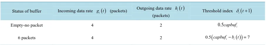
is zero. The dynamic nature of threshold index is shown in Table 1 where 20 packets are assumed as buffer capacity.

The possibility for congestion at node “i” is determined by comparing the buffer occupancy with the threshold index. The results show that

1) if b ti

( )

<δi

( )

t then there is no congestion in the node

2) if b ti

( )

=capbufi and g ti

( )

>h ti

( )

indicates congestion due to buffer overflow. Hence the probability of congestion occurrence for node “i” is given by

( )

(

)

(

( )

)

1

(

( )

( ) (

)

)

( )

1

x x

i n i

P δ t +x = p δ t +x +

∑

−₌p δ t +n

|

δ t + x−n =µ t (3)

The dynamic variable x

( )

i t

µ is considered as congestion_status. The value of x

( )

i t

µ varies from time to time and it indicates the probability for occurrence of congestion at node “i” when the buffer contains “x” num-ber of packets in excess to threshold index.

i

S is the set of neighbour nodes that are in the coverage area of node “i”. The probability for reception of a packet by node “i” from neighbour node “j” is given by

ij i

[image:4.595.87.540.636.713.2]

p = p ϕ (4)

Table 1. Instances of dynamic threshold index.

Status of buffer Incoming data rate g ti( ) (packets)

Outgoing data rate h ti( )

(packets)

Threshold index δi(t+1)

Empty-no packet 4 2 0.5capbufi

where j∈ ∀Si j, ϕ= Si and pi is the probability for node “i” to absorb packets from neighbours and 1− pi is the probability for dropping of packets.

The chance for a node to be in the vicinity of node “i” is Ci which is the coverage range of node “i” and it has a value of 1.

The probability for node “i” to have a neighbour set size of “φ” is determined by

(

)

1

(

)

1

1 1

n

i i i i

n

Pϕ p S ϕ C ϕCϕ

ϕ − − −   = = =_{ } − −

  (5) The probability expected by node “i” to receive packets from its neighbour is

( )

n₁ i 1

(

1

)

n

ij i i

i p

E P i p P C

nC ϕ ϕ=

= = − −

  _

 

∑

_  (6)

The intensity of congestion at a node is calculated from Equations (3) and (6) and it is propagated as feedback in backward direction to indicate the inception of congestion. The level of congestion is predicted by the value of µix

( )

t as follows:

1) if x

( )

0 i t

µ = No congestion

2) if µix

( )

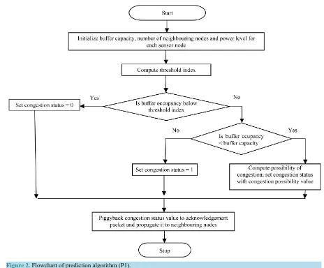
t >0 Congestion occurs and level of congestion in the node can also be indicated. The PCPA is denoted as (P1), for which the algorithm is given below:

Probability Based Congestion Prediction Algorithm (P1)

Initially

set ‘capbuf’ to maximum capacity of the buffer set ‘m’ to the set of neighbour nodes

set value of 'C' to power level of the node Congestion_occurrence_possibility()

// calculation of threshold index

h

(

capbuf b

)

g

δ = − ;

if (δ >b)

congestion_status =0 // no possibility for congestion else if

(

b>δ & &b<capbuf

)

x= −b δ ;

V =0;

for (i = 1; i<x; i++)

V = +V pow p m C

(

(

∗

)

∗ −

(

1 pow

(

(

1−C

)

,m

)

)

,i

)

;

congestion_status = V; //level of congestion possibility

end for

else

congestion_status = 1 //congestion end if

// propagate feedback about congestion to source piggyback ACK with congestion_status forward ACK to upstream nodes

This algorithm P1 is represented in terms of flow chart inFigure 2.

3.2. Rate Adjustment Based on Probabilistic Prediction

Each node in the network executes algorithm (P1) to determine the possibility of congestion. The µix

( )

t is ap- pended to the Acknowledgement (ACK) frame using piggybacking concept and it is propagated as feedback among upstream nodes. Hence impact of congestion is minimized in hop-by-hop manner and according to the

( )

x i t

[image:6.595.78.542.80.464.2]

Figure 2.Flowchart of prediction algorithm (P1).

The QOS allows to sort out the entire network traffic into an InElastic Real Time (IERT) and Elastic Non Real Time traffic (ENRT). Further ENRT traffic is divided into High Priority ENRT (HPENRT), Medium Prior-ity ENRT (MPENRT) and Low PriorPrior-ity ENRT (LPENRT) traffic. The relation among these traffic flows in terms of QOS parameters is given by

IERT HPENRT MPENRT LPENRT

delay ≤delay ≤delay ≤delay (7)

IERT HPENRT MPENRT LPENRT

throughput ≥throughput ≥throughput ≥throughput

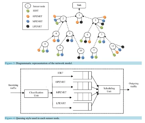
Figure 3shows the network model used for simulation. It has one sink and twelve sensor nodes represented as (1 to 12) and depict a classic WMSN with sensors of different nature. This model supports a single path communication. Each sensor node in the model collects data from real time inelastic traffic flow class and three categories of non real time traffic flow classes namely IERT, HPENRT, MPENRT, and LPENRT.

Figure 4shows the queuing style used in each node. Each traffic flow class has its own queue and to achieve discrimination among different traffic flow classes, each sensor node attaches a flow class label to every packet; therewith each incoming packet is appended to their respective queue.

The sensor node is assigned with two priorities: traffic flow class priority

( )

PFCi and location priority

( )

i L P .

It is assumed that each node has different source traffic flow classes. Let

( )

TSij represents the source priority

[image:7.595.71.549.79.484.2]

Figure 3.Diagrammatic representation of the network model.

Figure 4.Queuing style used in each sensor node.

For each node “i”, the value of traffic flow class priority

( )

PFCi is determined in Equation (8)

i i

FC j j

P =

∑

TS (8)

where “j” represents all categories of traffic flow classes such as IERT, HPENRT, MPENRT, and LPENRT. Generally in WSN, sensor nodes are set with variety of sensors and are geographically located in different places based on their importance. Hence these sensors need preferential treatment to attain dissimilar throughput. To attain this fairness, each sensor node is assigned with location priority

( )

PLi by the network administrator.

The local priority

( )

LPi of each node “i” is given in Equation (9)

i i i

L FC

LP =P ⋅P (9)

Considered D(i) as the child set of node “i”. Hence the overall priority

( )

OPi of each node is given by

( )

i l i

l D i

OP =

∑

_∈ OP +LP (10)

Probabilistic Prediction Based Rate Adjustment Algorithm (PPRAA)

The initialization of outgoing data rate is carried out as follows: Consider S

st

T is the service time taken by sink to service the current packet. The average service time is measured as the time which starts from sending of packet from network layer to MAC layer and ends with re-ceiving message by network layer about successful transmission of the packet by MAC layer. Formulating with exponential weighted sum,

Average service time,

(

1

)

S S S

st st st

T = −ω T + ⋅ω T (11)

where ω is a constant, 0≤ ≤ω 1. The output rate of sink node,

1 sink S st og T

= (12)

Substituting the value of Equation (12), the outgoing data rate

(

max

)

i

og for each child node “i” based on its

own overall priority

( )

i

OP and overall priority of sink node

(

sink

)

OP is given in Equation (13).

max i i sink sink OP og og OP  ₌  

 ⋅  (13) where sink

OP is the cumulative of overall priority of each child node of the sink node. Consider S sink

(

)

as the child set of sink node. The overall priority of sink node

(

OPsink

)

is calculated from Equation (14)

( )

sink j

j S sink

OP =

∑

_∈ OP (14)

The steps are repeated to determine the initial outgoing data rate of each node in the network.

Congestion prediction and rate adjustment

For each predetermined time period Tperiod, repeat the following steps at sink node:

Compute the possibility of congestion occurrence µsinkx

( )

t at the sink node as shown in Section 2.1.

The new outgoing data rate of each child node “i” of sink

(

ogouti

)

is calculated from Equation (15) which

will be propagated to each child node of sink.

( )

1 i

i i i x

out out out sink sink

OP

og og og t

OP µ

  

= −  ⋅ − 

 

  (15) For each predetermined time interval Tperiod (other nodes):

Compute the possibility of congestion occurrence x

( )

i t

µ at each parent node “i” as shown in Section 2.1.

The new outgoing data rate for each child node “j”

(

ogoutj

)

is determined by its parent node “i” as follows:

( )

1 j

j j j x

out out out i i

OP

og og og t

OP µ

= − _ ⋅ −_ __

 

  (16) The above is used by each node to determine its new outgoing data rate.

In this algorithm, for each predetermined time interval, the outgoing data rate for each sensor node is deter-mined by its parent node only and the outgoing data rate for each parent node is in turn deterdeter-mined by its own parent node. Since the sink has no parent node, its allowable outgoing data rate is determined from the inverse of its service time average.

The simulation of the present work has been carried out in NS2 simulator.

4. Results and Discussions

present work congestion intensity is predicted using probabilistic method based on incoming and outgoing data rate and buffer occupancy. Moreover the threshold value used for comparing buffer occupancy is dynamic, so that efficient prediction of congestion intensity and subsequent adjustment of outgoing data rate minimizes packet drops. The network model proposed also allocates resources among sensor nodes efficiently based on priority of the source data and location, thus maintaining a good throughput.

In the present work simulation as per the model mentioned inFigure 3 is carried out. The work is simulated for 30 runs with 75 seconds per run. During the process sensor nodes start sending data at the beginning of si-mulation run and finish it at the end of sisi-mulation run. The location priority of all sensor nodes is assumed as 1. The size of each packet is 250 bytes. The size of the buffer in every child is 75 packets and the size of buffer in sink is 125 packets. Table 2shows the parameters used for simulation.

The traffic flow classes that each sensor node has in the simulation model are shown in Table 3. It is assumed that each sensor node should have gathered data from all the traffic flow classes IERT, HPENRT, MPENRT, and LPENRT and their assigned weight values are correspondingly 7, 5, 3 and 1. The traffic flow class priority

( )

1 FC

P for node “1” which includes HPENRT and LPENRT traffic flow classes is determined as 5 + 1 = 6 (the weight of HPENRT is 5 and LPENRT is 1). For node 3 which includes all traffic flow classes, the traffic flow class priority

( )

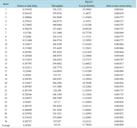
PFC3 is calculated as 7 + 5 + 3 + 1 = 16 (since the weights of IERT, HPENRT, MPENRT and LPENRT are 7, 5, 3 and 1 respectively).

The performance of the present approach during 30 simulation runs is evaluated for various parameters such as throughput, loss probability, sink-to-base station delay and source-to-sink delay and is tabulated inTable 4.

[image:9.595.146.481.435.706.2]

The results for the present work are also correlated with already existing two congestion control approaches EWPBRC and FEWPBRC (Figures 5-8) and the comparative result statement is shown in Table 5.

Table 5 shows the average of results obtained in 30 runs for various performance metrics for the existing works EWPBRC, FEWPBRC and proposed work PQACC. FromTable 5 it is clear that the average throughput achieved by PQACC is 9% higher than EWPBRC and 5.978% higher than FEWPBRC. The average sink-to- base station delay achieved by PQACC is 14.81% lower than EWPBRC and 11.51% lower than FEWPBRC. The average loss probability achieved by PQACC is 16.03% lower than EWPBRC and 11.69% lower than FEWPBRC. The average source-to-sink delay achieved by PQACC is 10.33% lower than EWPBRC and 7.05% lower than FEWPBRC.

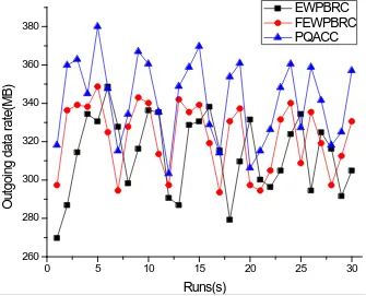
Figure 5.Throughput to base station from sink over runs.

0 5 10 15 20 25 30

260 280 300 320 340 360 380

O

ut

goi

ng dat

a r

at

e(

M

B

)

Runs(s)

[image:10.595.147.533.62.713.2]

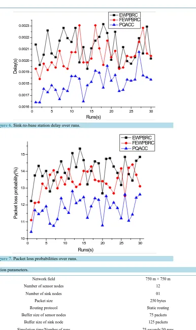
Figure 6. Sink-to-base station delay over runs.

[image:10.595.168.506.86.315.2]

Figure 7.Packet loss probabilities over runs.

Table 2. Simulation parameters.

Network field 750 m × 750 m

Number of sensor nodes 12

Number of sink nodes 01

Packet size 250 bytes

Routing protocol Static routing

Buffer size of sensor nodes 75 packets

Buffer size of sink node 125 packets

Simulation time/Number of runs 75 seconds/30 runs

0 5 10 15 20 25 30

0.0016 0.0017 0.0018 0.0019 0.0020 0.0021 0.0022 0.0023

D

el

ay

(s

)

Runs(s)

EWPBRC FEWPBRC PQACC

0 5 10 15 20 25 30

10 11 12 13 14 15

P

ac

ket

los

s pr

obabi

lit

y(

%

)

Runs(s)

[image:10.595.87.537.602.719.2]

[image:11.595.88.537.101.270.2]

Table 3. Status of traffic flow classes in each sensor node.

Sensor node no. IERT (W = 7) HPENRT (W = 5) MPENRT (W = 3) LPENRT (W = 1) Traffic flow class priority i

FC

P

Node 1 OFF ON OFF ON 6

Node 2 ON ON ON OFF 15

Node 3 ON ON ON ON 16

Node 4 OFF ON ON OFF 8

Node 5 OFF OFF ON ON 4

Node 6 ON ON OFF ON 13

Node 7 ON OFF ON OFF 10

Node 8 ON ON ON OFF 15

Node 9 ON OFF ON OFF 10

Node 10 OFF OFF ON ON 4

Node 11 ON OFF ON OFF 10

Node 12 ON ON ON ON 16

Table 4. Results in simulation runs for the present work.

Run# PQACC

Source-to-sink delay Throughput Loss probability Sink-to-base station delay

1 0.318182 318.1521 10.39962 0.001641

2 0.301435 359.8536 11.6875 0.001639

3 0.300866 362.9049 11.45454 0.001757

4 0.279221 344.9772 11.6553 0.001727

5 0.274892 380.0494 11.91288 0.001787

6 0.266576 347.6483 10.88258 0.001747

7 0.31784 315.1008 10.75758 0.001668

8 0.32684 334.3118 11.15151 0.001757

9 0.311688 366.9734 12.39583 0.001737

10 0.316017 360.5209 11.81629 0.001866

11 0.311802 335.4429 11.52651 0.001866

12 0.287081 303.2852 12.81439 0.001844

13 0.320346 348.8555 12.10606 0.001648

14 0.313853 358.8365 12.27273 0.001787

15 0.307587 369.6882 12.46023 0.001817

16 0.322511 328.7776 11.23674 0.001913

17 0.32684 314.0836 11.91288 0.001896

18 0.30303 353.751 12.39583 0.001767

19 0.298701 360.8707 12.29924 0.001956

20 0.316017 306.2586 10.78598 0.001826

21 0.299385 315.1008 12.52462 0.001876

22 0.307359 326.289 11.81818 0.001737

23 0.320346 348.1369 12.13826 0.001747

24 0.324675 360.5209 11.81629 0.001836

25 0.30303 327.27 11.20454 0.001826

26 0.305195 358.8365 12.62121 0.001836

27 0.284689 341.5456 11.06061 0.002075

28 0.323992 318.1521 11.42992 0.001872

29 0.318182 325.0494 12.42803 0.001856

30 0.302727 357.057 12.62121 0.001836

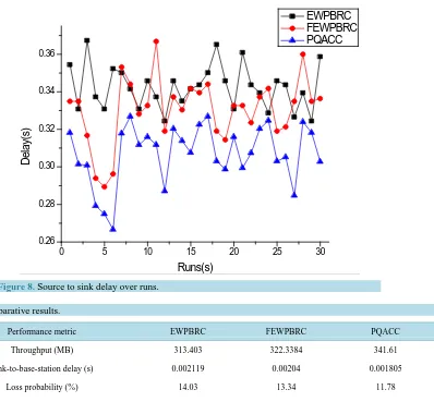
[image:11.595.89.541.297.720.2]

[image:12.595.139.537.79.448.2] [image:12.595.93.540.371.459.2]

Figure 8.Source to sink delay over runs.

Table 5. Comparative results.

Performance metric EWPBRC FEWPBRC PQACC

Throughput (MB) 313.403 322.3384 341.61

Sink-to-base-station delay (s) 0.002119 0.00204 0.001805

Loss probability (%) 14.03 13.34 11.78

Source-to-sink delay (s) 0.34243 0.33034 0.30703

Figure 5shows the comparison of throughput _ogsink

which is the total outgoing data rate of sink node to the base station, in each run. The average throughput is 313.403 MB for EWPBRC, 322.33 MB for FEWPBRC and 341.61 for the PQACC. From the results it is observed that PQACC is good compared with EWPBRC and FEWBPRC. The increase in average throughput is due to minimization of packet drops with efficient congestion prediction and effective allocation of network resources among sensor nodes.

Figure 6 shows the comparison of sink-to-base station delay of EWPBRC, FEWBPRC and PQACC. Sink- to-base station delay is the time taken by sink node for transmission of data to the base station. The average sink-to-base station delay is 0.002119 seconds for EWPBRC, 0.00204 seconds for FEWPBRC and 0.001805 seconds for the PQACC. The decrease in delay time is due to minimization of retransmissions by packet drops depicting the faster delivery of data packets.

Figure 7shows the comparison of packet loss probability for all three approaches. Packet loss probability is the ratio between the numbers of packets dropped in the network to number of packets transmitted by the sensor nodes. The average packet loss probability is 14.03% for EWPBRC, 13.34% for FEWPBRC and for PQACC it is 11.78%. PQACC has the minimum percentage of packet loss probability. The decrease in packet loss proba-bility is due to efficient prediction and adjustment of outgoing data rate of sensor nodes.

Figure 8 shows the relationship between source to sink delay and run. It is the time taken by each child node to forward data to the sink, in each run for EWPBRC, FEWPBRC and PQACC. The average values of source to sink delay are 0.34242 seconds, 0.33034 seconds and 0.30703 seconds for EWPBRC, FEWPBRC and PQACC respectively. The results show that the source to sink delay is minimum for PQACC. This decrease in delay time is due to effective allocation of network resources among sensor nodes and efficient determination of outgoing data rate for sensor nodes.

0 5 10 15 20 25 30

0.26 0.28 0.30 0.32 0.34 0.36

D

el

ay

(s

)

Runs(s)

5. Conclusion

The protocol PQACC, for congestion control is developed by considering the requirements of multimedia ap-plications on WMSNs. To achieve QOS for various types of data, each traffic type is set with a priority. The outgoing data rate of each source is adjusted based on the priority of data, predicted level of congestion and deployed location of the sensor nodes. The proposed approach allocates more network resources to high-priority traffic flow compared to low-priority traffic flow, so that real-time traffic gets preferential treatment over non- real-time traffic which is a requirement for WMSN. The threshold value used for comparing buffer occupancy to predict congestion intensity is dynamic, so that efficient prediction is achieved. The results from the simulation data for PQACC efficiently diminish the congestion for a better QOS. The probabilistic method used in the present study, for predicting the level of congestion gives good result compared with EWPBRC and FEWPBRC approaches. Hence an improvement is achieved in throughput, delay and packet loss of the network. This pro-posed approach can be employed in tracking systems and monitoring applications. In future the work can be op-timized using neuro-fuzzy approach.

References

[1] Chen, Y.L. and Lai, H.P. (2012) Priority-Based Transmission Rate Control with a Fuzzy Logical Controller in Wireless Multimedia Sensor Networks. Computers and Mathematics with Applications, 64, 688-698.

http://dx.doi.org/10.1016/j.camwa.2011.09.034

[2] Kafi, M.A., Djenouri, D., Ben-othman, J. and Badache, N. (2014) Congestion Control Protocols in Wireless Sensor Networks: A Survey. IEEE Communication Surveys and Tutorials, 16, 1369-1390.

http://dx.doi.org/10.1109/SURV.2014.021714.00123

[3] Yaghmaee, M.H. and Adjeroh, D.A. (2009) Priority-Based Rate Control for Service Differentiation and Congestion Control in Wireless Multimedia Sensor Networks. Computer Networks, 53, 1798-1811.

http://dx.doi.org/10.1016/j.comnet.2009.02.011

[4] Farooq, M.O. and Kunz, T. (2011) Wireless Multimedia Sensor Networks Test beds and State-of-the-Art Hardware: A Survey. Proceedings of Future Generation in Communication and Networking (FGCN), Jeju Island, South Korea, 1- 14.

[5] Akyildiz, I.F., Su, W., Sankarasubramaniam, Y. and Cayirci, E. (2002) Wireless Sensor Networks: A Survey.

Comput-er Networks, 38, 393-422. http://dx.doi.org/10.1016/S1389-1286(01)00302-4

[6] Sergiou, C., Vassiliou, V. and Paphitis, A. (2013) Hierarchical Tree Alternative Path (HTAP) Algorithm for Conges-tion Control in Wireless Sensor Networks. Ad Hoc Networks, 11, 257-272.

http://dx.doi.org/10.1016/j.adhoc.2012.05.010

[7] Flora, D.J., Kavitha, V. and Muthuselvi, M. (2011) A Survey on Congestion Control Techniques in Wireless Sensor Networks. Proceedings of International Conference on Emerging Trends in Electrical and Computer Technology

ICETECT, Nagercoil, 23-24 March 2011, 1146-1149.

[8] Sergiou, C., Antoniou, P. and Vassiliou, V. (2014) A Comprehensive Survey of Congestion Control Protocols in Wireless Sensor Networks. IEEE Communication Surveys and Tutorials, 16, 1839-1859.

http://dx.doi.org/10.1109/COMST.2014.2320071

[9] Ee, C.T. and Bajcsy, R. (2004) Congestion Control and Fairness for Many-to-One Routing in Sensor Networks.

Pro-ceedings of the 2nd International Conference on Embedded Networked Sensor Systems, Baltimore, 3-5 November

2004, 148-161. http://dx.doi.org/10.1145/1031495.1031513

[10] Kang, J., Zhang, Y. and Nath, B. (2007) TARA: Topology-Aware Resource Adaptation to Alleviate Congestion in Sensor Networks. IEEE Transactions on Parallel and Distributed Systems, 18, 919-931.

http://dx.doi.org/10.1109/TPDS.2007.1030

[11] Wan, C.-Y., Eisenman, S.B. and Campbell, A.T. (2003) CODA: Congestion Detection and Avoidance in Sensor Net-works. Proceedings of the 1st International Conference on Embedded Networked Sensor Systems, Los Angeles, 5-7 November 2003, 266-279. http://dx.doi.org/10.1145/958491.958523

[12] Wang, C., Sohraby, K., Lawrence, V., Li, B. and Hu, Y. (2006) Priority-Based Congestion Control in Wireless Sensor Networks. Proceedings of International Conference on Sensor Networks, Ubiquitous and Trustworthy Computing, 1, 22-31. http://dx.doi.org/10.1109/SUTC.2006.1636155

[13] Wang, C., Li, B., Sohraby, K., Daneshmand, M. and Hu, Y. (2007) Upstream Congestion Control in Wireless Sensor Networks through Cross-Layer Optimization. IEEE Journal on Selected Areas in Communications, 25, 786-795.

[14] Hull, B., Jamieson, K. and Balakrishnan, H. (2004) Mitigating Congestion in Wireless Sensor Networks. Proceedings

of the 2nd International Conference on Embedded Networked Sensor Systems, Baltimore, 3-5 November 2004, 134-

147. http://dx.doi.org/10.1145/1031495.1031512

[15] Rangwala, S., Gummadi, R., Govindan, R. and Psounis, K. (2006) Interference Aware Fair Rate Control in Wireless Sensor Networks. SIGCOMM Computer Communication Review, 36, 63-74.

http://dx.doi.org/10.1145/1151659.1159922

[16] Vedantham, R., Sivakumar, R. and Park, S.J. (2007) Sink-to-Sensors Congestion Control. Ad Hoc Networks, 5, 462- 485. http://dx.doi.org/10.1016/j.adhoc.2006.02.002

[17] Annie Uthra, R., Kasmir Raja, S.V., Jeyasekar, A. and Anthony Lattanze, J. (2014) A Probabilistic Approach for Pre-dictive Congestion Control in Wireless Sensor Networks. Journal of Zhejiang University—Science C (Computers &

Electronics), 15, 187-199. http://dx.doi.org/10.1631/jzus.C1300175

[18] Rajan, A.U., Kasmir Raja, S.V., Jeyasekar, A. and Anthony Lattanze, J. (2015) Energy-Efficient Predictive Congestion Control for Wireless Sensor Networks. IET Wireless Sensor Systems, 5, 115-123.

http://dx.doi.org/10.1049/iet-wss.2013.0101