Hedge Ratios in South African Stock Index Futures

(1)

Munich Personal RePEc Archive

Hedge Ratios in South African Stock

Index Futures

Degiannakis, Stavros and Floros, Christos

Department of Economics, University of Portsmouth, Portsmouth

Business School, Portsmouth, Portland Street, PO1 3DE, United

Kingdom

2010

Online at

https://mpra.ub.uni-muenchen.de/96301/

(2)

1 | P a g e

Hedge Ratios in South African Stock Index Futures

Stavros Degiannakis and Christos Floros*

Department of Economics, University of Portsmouth, Portsmouth Business School, Portsmouth,

Portland Street, PO1 3DE, United Kingdom

*Corresponding author: Email: Christos.Floros@port.ac.uk, Tel: +44 (0) 2392 844244

Abstract

This paper examines hedging in South African stock index futures market. The

hedge ratios are estimated by six econometric techniques: the standard OLS

regression, simple and vector error correction models, the ECM with generalised

autoregressive heteroskedasticity (GARCH) as well as time-varying CCC-ARCH and

Diag-BEKK ARCH models. The empirical results show that the ECM-GARCH

model (capturing volatility clustering) provides best hedging ratios, while

CCC-ARCH is superior to OLS, ECM and VECM. We conclude that there is not a unique

model specification for measuring hedge ratios. For each market (emerging and mature), a model’s comparative analysis must be conducted in order to extract the best performing model.

JEL Classification: G13, G15.

(3)

2 | P a g e

I. INTRODUCTION AND THEORY

Hedging is the most important function of futures markets. It is concerned

with the management of risk. Theory description of hedging include Working (1953),

Johnson (1960), Stein (1961), Rutledge (1972), Ederington (1979) and Floros and

Vougas (2004). In general, hedging is the action taken by a buyer or seller to protect

his/her business or assets against a change in prices, see Floros and Vougas (2004).

From the theoretical point of view, there are three goals of hedging: risk

minimisation, profit maximisation, and the portfolio approach, see Rutledge (1972).

Hedging is carried out to (i) eliminate risk due to adverse price fluctuation, (ii) reduce

risk due to adverse price moves, (iii) profit from changes in the basis, and (iv)

maximise expected return for a given risk and minimise risk for a stated return

(Sutcliffe, 1993).

Stock index futures contracts can be used to hedge the risk. Hedging uses

futures markets to reduce risk of a cash (spot) market position. According to Hull

(2000, p. 66), when the relationship between the cash price and the price of a futures

contract is very close, the hedge is more effective. However, because this relationship

is usually not perfect (spot and futures positions do not move together), the hedge is a

cross-hedge. In this case, the hedger should trade the right number of futures contract

to control the risk. In other words, the determination of the optimal hedge ratio1

(minimum variance hedge ratio, or MVHR) is required. MVHR is the optimal amount

of futures bought or sold expressed as a proportion of the cash position. It is important

for the hedger to be able to identify the number of contracts needed to hedge the

portfolio. Thus, the hedge ratio (HR) will be used, so one can choose the right number

of futures contracts minimising risk. The HR is the number of futures contracts

bought, or sold, divided by the number of spot contracts whose risk is being hedged.

Several measures have been proposed for the HR computation. Usually, the

HR is estimated from an OLS regression of cash on futures prices. The method is

introduced by Ederington (1979), and Anderson and Danthine (1980). The slope

coefficient of the OLS regression is the MVHR, which is constant over time. An

alternative estimation of the optimal HR is based on the phenomenon that cash and

futures prices display volatility clustering, and, hence, GARCH models are to be

1_{Optimal hedge ratio is derived from the optimisation of certain objective functions, such as}

(4)

3 | P a g e

preferred. These models are used for estimating heteroscedastic optimal hedge ratios,

see Cecchetti et al. (1988) and Floros and Vougas (2004). Furthermore, several

studies use error correction models (ECM) to estimate the hedge ratios, see Chou et

al. (1996) and Lien (1996). Other papers use error correction terms with a

time-varying risk structure when analysing the spot-futures relationship, see Kroner and

Sultan (1993), and Lien and Tse (1999). According to Lee and Chien (2010), various

econometric models give different conclusions when estimate HR. Miffre (2004)

shows that the conditional OLS model outperforms the OLS and GARCH models,

while Alexander and Barbosa (2007) find no evidence that time-varying conditional

covariance and ECM can improve upon the OLS hedge ratio. Recently, Hsu et al.

(2008) suggest that copula-based GARCH models perform more effectively than

OLS, CCC-GARCH and DCC-GARCH models (for more information about the

performance of various econometric models for HR estimation see Lee and Chien,

2010).

Lien and Zhang (2008) summarise theoretical and empirical research on the

roles and functions of emerging derivatives markets and report mixed results. The

present paper focuses on model specification and empirical comparison of several

models for HR estimation using data from an emerging market; the South African

futures market (FTSE/JSE 40 Index). The traditional regression model OLS, the

ECM, the VECM, and the ECM-GARCH models as well as the dynamic CCC-ARCH

and Diag-BEKK ARCH models are employed. According to authors’ knowledge this

is the only empirical investigation using data from South African futures market.

The manuscript is organised as follows: Section II shows an overview of

econometric models employed for estimating hedge ratios. Section III describes the

data, and Section IV presents the empirical results from the econometric models.

Section V discusses a comparison between models and Section VI concludes the

paper and summarises our findings.

II. METHODOLOGY

The futures hedge ratios are mainly calculating via the OLS regression model.

Butterworth and Holmes (2000) estimated the (ex post) MVHR using OLS, by

regressing the first order log difference in the spot prices, St, against the first order

(5)

4 | P a g e

t t

t c b F u

S    



) , 0 ( ~ 2

N

ut ,

(1)

whereSt logSt logSt1, Ft logFtlogFt1. The coefficient b is the hedge

ratio2.

Nevertheless, the former model specification assumes the absence of

auto-correlation and heteroskedasticity in log-returns. There is substantial evidence in

financial literature to suggest that financial time series do not comply with the

assumption of uncorrelated and homoskedastic returns to financial instruments. Chou

et al. (1996), following the method proposed by Engle and Granger (1987), estimated the hedge ratio, using an error correction model (ECM). Assuming the series are

co-integrated, there exists an ECM of the form:

t t t

t t

t c a b F F S u

S         

 ˆ_₁ ₁ _₁ ₁ _₁ ,

) , 0 ( ~ 2

N

ut ,

(2)

where ˆt1St1



cˆ0bˆ0Ft1



. The coefficient b is the hedge ratio.

In addition, one may use ECM with time varying terms in the variance

equation (GARCH errors), or:

t t t

t t

t c a b F F S u

S         

 ˆ_1 1 _1 1 _1 ,

t t

t z

u 

2 1 1 2

1 1 0 2

  



 t t

t a au 



 

0,1

~ N

z_t

(3)

An iterative procedure is used based upon the method of Marquardt algorithm.

Heteroskedasticity Consistent Covariance option is used to compute quasi-maximum

likelihood covariances and standard errors using the methods described by Bollerslev

and Wooldridge (1992). This is normally used if the residuals are not conditionally

normally distributed (for more details about GARCH models see Xekalaki and

Degiannakis, 2010).

2_{For all the models, the Newey and West (1987) heteroskedasticity and autocorrelation consistent}

(6)

5 | P a g e

Ghosh (1993) and Lien (1996) calculated the optimal hedge ratio using a

VECM specification: t S t t t S

t a F S u

S  ˆ ₁ ₁₁ ₁ ₁₁ ₁ _,

 _  _  _ , (4)

t F t t t F

t a F S u

F  ˆ ₁ ₁₂ ₁ ₁₂ ₁ _,

 _  _  _ , (5)

where _

                          2 , , 2 , , , 0 0 ~ F F S F S S t F t S N u u    

. The hedge ratio is calculated as 1

F S  , where 2 2 , F S F S   

  is the correlation coefficient between uS,t and uF,t, and S and

F

 are the standard deviations of uS,t and uF,t, respectively.

Moreover, we proceed to the estimation of the optimal hedge ratio using two

bivariate ARCH specifications. An ARCH system of 2 regression equations is

defined:







, ,..., , ,...



, , ~ | 2 1 2 1 1          t t t t t t t t t t t g N I u u H H H H 0 u u x B y (6) where                                          t F t S t t t F S t t t t t u u S F a a F S , , 1 1 1 12 12 11 11 ˆ      u x B

y , (7)

1



t

I is the available information set, N



0,Ht



is the bivariate normal distribution with

 

u_t 0

E , conditional mean, and V

 

ut Ht, conditional variance, respectively.

We are based on two successfully applied versions of the bivariate ARCH

process; Bollerslev's (1990) constant conditional correlation, or CCC-ARCH, model,

and Baba's et al. and Engle and Kroner's (1995) diagonal BEKK, or Diag-BEKK

ARCH, model.

In the CCC-ARCH model the conditional variance of ut is decomposed as:

2 / 1 2 / 1 t t

t Σ CΣ

H  , (8)

where _

      t F t S t , , 2 / 1 0 0  

Σ is the diagonal matrix with the conditional standard

deviations along the diagonal, and _

      1 1  

(7)

6 | P a g e

correlations. The conditional standard deviations are computed as univariate

GARCH(1,1) models: 2 1 , 1 , 1 2 1 , 1 , 1 0 , 1 2

,t   St  St

S a  u  

 , (9)

2 1 , 1 , 2 2 1 , 1 , 2 0 , 2 2

,t   Ft  Ft

F a  u  

 , (10)

and the conditional covariance is computed as:

t F t S t F

S, ,  , ,

  . (11)

The hedge ratio is calculated as

t F t S t F t F S , , 2 , , ,       .

In the Diag-BEKK ARCH model the conditional variance of ut is decomposed as:

            

 _ _ _ ₂

, , , , , 2 , 1 1 1 1 1 1 1 t F t F S t F S t S t t t

t  

  B H B A u u A A A

H ₀ ₀ . (12)

The conditional variances are computed as GARCH(1,1) models in forms follow:

1 , 1 , 1 2 1 , 1 , 1 , 1 1 , 1 , 1 2 1 , 1 , 1 , 1 1 , 1 , 0 2 ,   

St a a uSt_a  St_ , (13)

2 , 2 , 1 2 1 , 2 , 2 , 1 2 , 2 , 1 2 1 , 2 , 2 , 1 2 , 2 , 0 2 ,   

_F_t a a u_F_t_a  _F_t_ , (14)

and the conditional covariance is computed as:

2 , 2 , 1 1 , , 1 , 1 , 1 2 , 2 , 1 1 , 1 , 1 , 1 , 1 2 , 1 , 0 , ,   

SFt a a uSt_uFt_a  SFt_ . (15)

The hedge ratio is calculated as ₂

, , , t F t F S  

. For technical details about the aforementioned

bivariate ARCH models the interested reader is referred to Xekalaki and Degiannakis

(2010).

III. DATA DESCRIPTION

This study employs 1043 trading days on the FTSE/JSE Top 40 stock index

and stock index futures contract for the period 2 January 2002 to 28 February 2006.

Closing prices for the spot index were obtained from DataStream International, while

closing futures prices were obtained from the official webpage of the South African

Futures Exchange, or SAFEX (http://www.safex.co.za).

FTSE/JSE Top 40 stock index consists of the largest 40 companies ranked by

full market capitalisation (value) that is before the application of any weighting in the

All Share Index. The futures contract is the FTSE/JSE’s Top 40 future nearest to

(8)

7 | P a g e

to the nearby contract because almost all trading volume is in the near month so that

liquidity is much great in that contract compared with the far contract.

The futures contracts are quoted in the same units (South African Rand) as the

underlying index without decimals, with the price of a futures contract or contract size

being the quoted number (index level) multiplied by the contract multiplier, which is

R10 for the contract. Futures expiry months are March, June, September and

December. The stock index futures contract is cash-settled and marked to market on

the last trading day, which is at 15:40 South African time on the third Thursday in the

delivery or expiration month. The formal futures exchange was established in 1988 as

well as the SAFEX clearing company. For more details about the South African

market, see Motsa (2006) and Floros (2009).

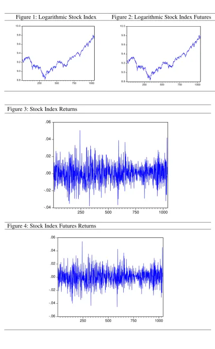
Figures 1 and 2 present the plots of logarithmic FTSE/JSE Top 40 stock index

and stock index futures, respectively. Figures 3 and 4 show the behaviour of returns of

both indices over time, indicating volatility clustering or pooling in FTSE/JSE Top 40

spot and futures returns.

<< Figure 1 about here >>

IV. EMPIRICAL RESULTS

First, we apply unit root tests for log-stock prices and log-futures prices for

FTSE/JSE Top 40. Augmented Dickey and Fuller (1979), or ADF test statistic, and

Phillips and Perron (1988), or PP test statistic, indicate that both series are I(1).

Cointegration are used to confirm whether there exists such a cointegrating structure between spot and futures markets. Johansen’s (1988, 2004) approach suggests that

spot and futures are cointegrated, with one cointegration relationship3. Thus, there

exists a linear combination of the South African spot and futures prices.

A. The Conventional Approach - OLS Regression

The optimal hedge ratio can be derived from the regression in equation (1),

where the returns to holding spot asset are regressed on the returns to holding the

hedging instruments. Table 1 presents the results for FTSE/JSE Top 40 index. The

hedge ratio is 0.9043, and it is significantly less than unity.

(9)

8 | P a g e

<< Table 1 about here >>

B. An Error Correction Approach

In our case, S and F are cointegrated, and therefore, the optimal hedge ratio can be calculated from an error correction model, see equation (2). We apply an ECM

to obtain alternative estimates for the hedge ratio, so we can compare them with the

ones obtained from the conventional method. The results are reported in Table 2.

The results show a hedge ratio of 0.9150 for FTSE/JSE Top 40. The hedge

ratio coefficient in the hedge equation (ECM) is significantly less than unity at any

level of significance. Comparing estimated hedge ratio, we conclude that the hedge

ratio estimated by equation (2) is greater than the one estimated by equation (1). This

implies that the conventional model under-estimates the number of futures contracts

needed to hedge the spot portfolio. This is not in line with Floros and Vougas (2004),

who provided evidence that in the case of the Greek stock market the FTSE/ASE-20

hedge ratio estimated by the ECM is less than that obtained from the OLS method.

C. An Error Correction Approach with GARCH Errors

The ECM specification, in equation (3), is also taken into consideration under

the assumption of time varying conditional variance. The coefficient b equals to

0.9212.

D. A Vector Error Correction Approach

If spot and futures prices are cointegrated, we can use a Vector Error

Correction Model (VECM) to estimate hedge ratio. The hedge ratio is calculated as

2 ,

F F S

h  

 . From equations (4) and (5), S,F is the covariance coefficient between the

innovations uS,t and uF,t, and S and F are the standard deviations of uS,t and

t F

u _, , respectively. Thus, the hedge ratio from VECM is calculated as

9143 . 0 000140 .

0

000128 .

0

2

, _ _



F F S

h  

. The estimation of the model is presented in Table 4.

The hedge ratio estimated from VECM, is close to the one obtained from ECM. In the

studies of Ghosh (1993) and Floros and Vougas (2004) the hedge ratios estimated

from VECM were greater than the ones obtained from OLS and ECM specifications.

(10)

9 | P a g e

E. The CCC-ARCH Model

The fifth model for estimating hedge ratio is by employing VECM model with

time varying conditional variances and covariance. To incorporate both short- and

long-run information of data, we model the mean equation (first moment) with an

error correction model, and in addition, we take into account heteroscedastic

variances and covariances (to capture volatility clustering), by modelling the

conditional variance matrix with Bollerslev's (1990) constant conditional correlation

framework.

Table 5 reports the results from CCC-ARCH model. Figure 5 plots the hedge

ratios across time. The average hedge ratio is 0.9169 for FTSE/JSE Top 40 index.

F. The Diag-BEKK ARCH Model

The last model for estimating hedge ratio is the DIAG-BEKK ARCH model.

Table 6 reports the estimation of the Diag-BEKK ARCH model. Figure 6 plots the

hedge ratios across time. The average hedge ratio is 0.9074 for FTSE/JSE Top 40

index. Hence, the hedge ratio estimated by CCC-ARCH model is greater than the one

obtained from that model. So, the hedge ratio estimated by CCC-ARCH model should

be more efficient in reducing risk of spot prices.

V. MODELS COMPARISON

Table 7 shows the hedge ratios estimated from the six econometric models.

The hedge ratio estimated by the ECM-GARCH model performs better in terms of

hedging. It is greater than the ones obtained from OLS, ECM and VECM. Hence,

hedgers need more futures contracts to reduce the market risk of their cash portfolios

(their losses are going to be reduced substantially). So, the hedge ratio estimated by

ECM-GARCH model should be more efficient in reducing risk of spot prices.

Furthermore, this implies that all other constant models (OLS, ECM and VECM)

under-estimate the number of futures contracts needed to hedge spot prices.

Therefore, hedge ratio estimated by ECM-GARCH significantly improves hedging.

(11)

10 | P a g e

models, and therefore this hedge ratio should provide better hedging (ECM-GARCH

performs well in terms of variance reduction).

Furthermore, we find that the dynamic hedge ratios obtained from the

CCC-ARCH and Diag-BEKK CCC-ARCH models have a sample mean less than unity, but

greater than the constant hedge ratios obtained from the traditional OLS and ECM. In

particular, the hedge ratio estimated from CCC-GARCH is greater than those from

OLS, ECM and VECM, while the hedge ratio obtained from the Diag-BEKK ARCH

is greater than that from the simple OLS and ECM. These estimates suggest that the

naive 1:1 hedging strategy is inappropriate; this is in line with Yang and Allen (2004).

We should note that the hedge ratio series obtained from CCC-ARCH and

Diag-BEKK ARCH are time varying hedge ratios, which, in turn, incorporates a

time-varying conditional correlation coefficient between the spot and futures prices and,

hence, generates more realistic time-varying hedge ratios (Yang and Allen, 2004).

Even though the sample mean hedge ratio form the Diag-BEKK ARCH model is

smaller in magnitude from the ones obtained from the traditional constant models

(ECM, VECM and ECM-GARCH), the average time-varying hedge ratio is just an indicative figure which doesn’t represent the actual hedge ratios from all time periods. The fact that time-varying models capture time-varying hedge ratios with success,

shows that these dynamic models are somewhat superior to the traditional models (in

particular to the OLS, ECM and VECM). Similarly, the mean of the time-varying

CCC-GARCH hedge ratio is larger than those derived from the simple OLS, the ECM

and the VECM, which means that the constant hedge ratios would lead to a smaller

than optimal hedging position (Sim and Zurbruegg, 2001).

VΙ. SUMMARY AND CONCLUSIONS

Futures contracts can be a very effective risk management instrument due to

its high liquidity and low transaction cost (Lien and Shrestha, 2010). When using

stock index futures for hedging (a technique to minimise risk), we require estimates of

the so-called hedge ratio. Various approaches for risk minimisation lead to different

estimation approaches and conclusions for the (optimal) hedge ratio. According to

Ghosh (p. 751, 1993), "Underestimating the optimal hedge ratio results in a

(12)

11 | P a g e

suboptimal hedge is significantly reduced and helps to reduce the impact of the costs of hedging".

In this paper, we focus on model specification and empirical comparison for

(optimal) hedge ratio estimation using data from South African futures market (an

emerging market). We examine the behaviour of futures prices from FTSE/JSE Top

40 index by employing six econometric methods, which include: the traditional OLS

regression model, ECM, ECM-GARCH, VECM, CCC-ARCH, and Diag-BEKK

ARCH models. The empirical results show that GARCH framework is superior to

traditional hedging models (OLS, ECM and VECM). It is found that the traditional

models underestimate the number of futures contracts, needed to hedge the spot

portfolio. In other words, portfolio managers can incur significant loss by using

traditional (constant) models.

In particular, we find that hedge ratio, estimated by ECM-GARCH, is greater

than the hedge ratio estimated by the other methods. We show that the FTSE/JSE Top

40 index hedge ratio estimated by ECM-GARCH significantly improves hedging. It is

superior to the other models implying better hedging; therefore, the hedge ratio

derived from ECM-GARCH is more effective in controlling and reducing risk of the

cash portfolio (Ghosh and Clayton, 1996). This indicates that a financial analyst or

trader whose portfolio includes the South Africa stock market should select the

optimal spot portfolio to be hedged and minimise risk exposure by estimating the

ECM-GARCH model.

This hedge ratio is more efficient than those estimated by all other techniques;

we also confirm that the constant hedge ratio derived from OLS is unable to recognise

the trend in the spot and futures changes (Park and Switzer, 1995). The

ECM-GARCH performs better than the other hedge ratios in terms of capturing conditional

variances (spot and futures changes). We show that hedgers in South African stock

index futures are able to estimate the number of futures contracts needed using an

ECM-GARCH model to reduce losses as well as overall costs of hedging.

However, we should note that the hedging strategy using the time-varying

model (CCC-ARCH) is superior to the traditional methods (OLS, ECM and VECM).

This is in line with Park and Switzer (1995). In particular, the mean of the

time-varying hedge ratios is larger than that derived from the simple models above, which

means that the simple hedge ratios would lead to a smaller than optimal hedging

(13)

12 | P a g e

Hence, we reach to a different conclusion in comparison to other similar

studies; e.g. the Greek emerging market, see Floros and Vougas, 2004. Therefore,

there is not a unique model specification for all the markets. For each market (emerging and mature), a model’s comparative analysis must be conducted in order to extract the best performing model.

Future research should evaluate the hedging effectiveness of the constant and

time-varying hedge ratios, measured in terms of ex-ante and ex-post risk-return

trade-off at various forecasting horizons, for several emerging markets across geographies

(14)

13 | P a g e

REFERENCES

Alexander, C., and Barbosa, A. (2007),' Effectiveness of minimum-variance hedging:

The impact of electronic trading and exchange-traded funds', Journal of Portfolio

Management, 32:46–59.

Anderson, R. W., and Danthine, J. P. (1980), ‘Hedging and joint production: theory

and illustrations’, Journal of Finance, 35:489-497.

Baba, Y., Engle, R.F., Kraft, D. and Kroner, K.F. (1990). Multivariate Simultaneous

Generalized ARCH. Department of Economics, University of California, San

Diego, Mimeo.

Bollerslev, T. (1990), 'Modeling the Coherence in Short-Run Nominal Exchange

Rates: A Multivariate Generalized ARCH Approach', Review of Economics and

Statistics, 72:498-505.

Bollerslev, T. and Wooldridge, J. M. (1992), ‘Quasi-maximum likelihood estimation and inference in dynamic models with time varying covariances’, Econometric Reviews, 11:143-172.

Butterworth, D., and Holmes, P. (2000), ‘Ex ante hedging effectiveness of UK stock

index futures contracts: evidence for the FTSE 100 and FTSE Mid 250 contracts’,

European Financial Management, 6:441-457.

Cecchetti, S. G., Cumby, R. E., and Figlewski, S. (1988), ‘Estimation of optimal

futures hedge’, Review of Economics and Statistics, 70:623-630.

Chou, W. L., Denis, K. K. F. and Lee, C. F. (1996), ‘Hedging with the Nikkei index

futures: the conventional model versus the error correction model’, Quarterly

Review of Economics and Finance, 36:495-505.

Dickey, D.A. and W.A. Fuller (1979), 'Distribution of the Estimators for

Autoregressive Time Series with a Unit Root', Journal of the American Statistical

Association, 74:427–431.

Ederington, L. (1979), ‘The hedging performance of the new Futures markets’,

Journal of Finance, 34:157-170.

Engle, R. F., and Granger, C. W. J. (1987), ‘Cointegration and error correction:

representation, estimation and testing’, Econometrica, 55:251-276.

Engle, R.F. and Kroner, K.F. (1995), 'Multivariate Simultaneous Generalized ARCH',

(15)

14 | P a g e

Floros, C., and Vougas, D. V. (2004), ‘Hedge ratios in Greek Stock Index Futures Markets’, Applied Financial Economics, 14(15):1125-1136.

Floros, C. (2009), ‘Price Discovery in the South African Stock Index Futures Market’,

International Research Journal of Finance and Economics, 34:148-159.

Ghosh, A. (1993), ‘Hedging with stock index futures: estimation and forecasting with

error correction model’, Journal of Futures Markets, 13:743-752.

Ghosh, A., and Clayton, R. (1996), ‘Hedging with international stock index futures: an intertemporal error correction model’, Journal of Financial Research, XIX:477-491.

Hansen, P.R. (2005), ‘A Test for Superior Predictive Ability’, Journal of Business and Economic Statistics, 23:365-380.

Hsu, C. C., Tseng, C. P. and Wang, Y. H. (2008), 'Dynamic hedging with futures: A

copulabased GARCH model', Journal of Futures Markets, 28:1095–1116.

Hull, J. C. (2000), Options, Futures, and Other Derivatives, Fourth Edition,

Prentice-Hall International, Inc.

Johansen, S. (1988), ‘Statistical Analysis of Cointegrating Vectors’, Journal of

Economic Dynamics and Control, 12:231-54.

Johansen, S. (2004), ‘The interpretation of cointegrating coefficients in the cointegrated vector autoregressive model’, Oxford Bulletin of Economics and Statistics.

Johnson, L. (1960), ‘The theory of hedging and speculation in commodity futures’,

Review of Economic Studies, 27:139-151.

Kroner, K. F., and Sultan, J. (1993), ‘Time varying distribution and dynamic hedging

with foreign currency futures’, Journal of Financial and Quantitative Analysis, 28:

535-551.

Lee, H-C., and Chien, C-Y. (2010), 'Hedging performance and stock market liquidity:

evidence from the Taiwan Futures Market', Asia-Pacific Journal of Financial

Studies, 39:396-415.

Lien, D. D. (1996), ‘The effect of the cointegrating relationship on futures hedging: a

note’, Journal of Futures Markets, 16:773-780.

Lien, D., and Shrestha, K. (2010), ‘Estimating optimal hedge ratio: a multivariate

skew-normal distribution approach’, Applied Financial Economics, 20:627-636.

Lien, D., and Tse, T. K. (1999), ‘Fractional Cointegration and Futures Hedging’,

(16)

15 | P a g e

Lien, D., and Zhang, M. (2008), 'A survey of emerging derivatives markets',

Emerging Markets Finance and Trade, 44(2):39-69.

Miffre, J. (2004), 'Conditional OLS minimum variance hedge ratios', Journal of

Futures Markets, 24:945–964.

Motsa, S. (2006), “Estimation of futures hedge ratios in South African futures exchange”, MSc dissertation, University of Portsmouth.

Newey, W. and West, K. (1987), A simple positive semi-definite, heteroskedasticity

and autocorrelation consistent covariance matrix, Econometrica, 55:703–708.

Park, T. H., and Switzer, L. N. (1995), ‘Time-varying distributions and the optimal

hedge ratios for stock index futures’, Applied Financial Economics, 5:131-137.

Phillips, P.C.B. and P. Perron (1988), 'Testing for a Unit Root in Time Series

Regression', Biometrika, 75:335–346

Rutledge, D. J. S. (1972), ‘Hedgers’ demand for futures contracts: a theoretical

framework with applications to the United States soybean complex’, Food

Research Institute Studies, 11:237-256.

Sim, A-B., and Zurbruegg, R. (2001), ‘Optimal hedge ratios and alternative hedging

strategies in the presence of cointegrated time-varying risks’, European Journal of

Finance, 7:269-283.

Stein, J. L. (1961), ‘The simultaneous determination of spot and futures prices’,

American Economic Review, 51:1012-1025.

Sutcliffe, C. M. S. (1993), Stock index futures: theories and international evidence,

Chapman & Hall.

Working, H. (1953), ‘Futures trading and hedging’, American Economic Review,

43:314-343.

Xekalaki, E. and Degiannakis, S. (2010), ARCH models for financial applications,

John Wiley.

(17)

16 | P a g e

TABLES AND FIGURES

Table 1. Estimated parameters of the regression model in equation (1). The coefficient to

standard error ratios are reported in brackets.









t t

t c b F u F u

S       

 0.000050.72 0.904363.44 .









₁





 

₁





₁ ,

1 1 1 1 1 . 72 . 3 21 . 0 51 . 4 23 . 0 80 . 74 915 . 0 ˆ 71 . 4 00001 . 0 34 . 0 00003 . 0 ˆ t t t t t t t t t t t u S F F u S F F b a c S                                

where ˆt_₁ St_₁



cˆ₀bˆ₀Ft_₁



St_₁



75.97



5.30



1.002



784.3



Ft_₁



.

 





₁





 

₁





₁ ,

1 1 1 1 1 50 . 5 25 . 0 43 . 5 24 . 0 34 . 98 921 . 0 ˆ 44 . 3 00002 . 0 35 . 1 00018 . 0 ˆ t t t t t t t t t t t u S F F u S F F b a c S                                

 





2

1 2 1 2 1 1 2 1 1 0 2 . 6 . 109 98 . 0 80 . 1 018 . 0 14 . 0 09 5 .

6  



     



 _t _t _t _t

t a au  E u 



where ˆt₁St₁



cˆ₀bˆ₀Ft₁



St₁



75.97



5.30



1.002



784.3



Ft₁



.

Table 4. Estimated parameters of the CCC-ARCH model. The coefficient to standard error ratios are

reported in brackets.

[image:17.595.35.566.559.655.2]

(18)

17 | P a g e

Table 5. Estimated parameters of the CCC-ARCH model. The coefficient to standard error ratios are

reported in brackets.













 









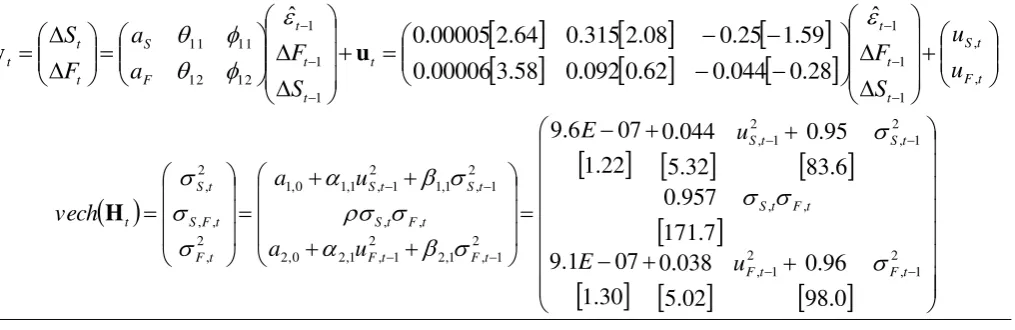
_ _                                                           t F t S t t t t t t t F S t t t u u S F S F a a F S , , 1 1 1 1 1 1 12 12 11 11 ˆ 28 . 0 044 . 0 62 . 0 092 . 0 58 . 3 00006 . 0 59 . 1 25 . 0 08 . 2 315 . 0 64 . 2 00005 . 0 ˆ       u y

 

   

 





   





                                                          0 . 98 96 . 0 02 . 5 038 . 0 30 . 1 07 1 . 9 7 . 171 957 . 0 6 . 83 95 . 0 32 . 5 044 . 0 22 . 1 07 6 . 9 2 1 , 2 1 , , , 2 1 , 2 1 , 2 1 , 1 , 2 2 1 , 1 , 2 0 , 2 , , 2 1 , 1 , 1 2 1 , 1 , 1 0 , 1 2 , , , 2 , t F t F t F t S t S t S t F t F t F t S t S t S t F t F S t S t u E u E u a u a vech                H

Table 6. Estimated parameters of the Diag-BEKK ARCH model. The coefficient to standard error ratios

are reported in brackets.

[image:18.595.50.558.136.301.2]

 













 

_ _                                                           t F t S t t t t t t t F S t t t u u S F S F a a F S , , 1 1 1 1 1 1 12 12 11 11 ˆ 81 . 0 084 . 0 07 . 0 007 . 0 09 . 5 00003 . 0 39 . 1 145 . 0 21 . 2 221 . 0 26 . 1 000008 . 0 ˆ       u y

 



  





 

   





                                                                       8 . 186 978 . 0 978 . 0 40 . 6 185 . 0 185 . 0 11 . 2 06 6 . 1 978 . 0 968 . 0 185 . 0 207 . 0 33 . 2 06 0 . 2 5 . 144 968 . 0 968 . 0 08 . 9 207 . 0 207 . 0 57 . 2 06 5 . 2 2 1 , 2 1 , 1 , , 1 , 1 , 2 1 , 2 1 , 2 , 2 , 1 2 1 , 2 , 2 , 1 2 , 2 , 1 2 1 , 2 , 2 , 1 2 , 2 , 0 2 , 2 , 1 1 , , 1 , 1 , 1 2 , 2 , 1 1 , 1 , 1 , 1 , 1 2 , 1 , 0 1 , 1 , 1 2 1 , 1 , 1 , 1 1 , 1 , 1 2 1 , 1 , 1 , 1 1 , 1 , 0 2 , , , 2 , t F t F t F S t F t S t S t S t F t F t F S t F t S t S t S t F t F S t S t u E u u E u E a u a a a u u a a a u a a vech                H

Table 7. Hedge ratios estimated from the six models.

OLS 0.9043

ECM 0.9150

ECM-GARCH 0.9212

VECM 0.9143

CCC-ARCH 0.9169

[image:18.595.44.557.356.715.2]

(19)

[image:19.595.75.519.56.775.2]

18 | P a g e

Figure 1: Logarithmic Stock Index Figure 2: Logarithmic Stock Index Futures

8.8 9.0 9.2 9.4 9.6 9.8 10.0

250 500 750 1000 8.8

9.0 9.2 9.4 9.6 9.8 10.0

250 500 750 1000

Figure 3: Stock Index Returns

-.04 -.02 .00 .02 .04 .06

250 500 750 1000

Figure 4: Stock Index Futures Returns

-.06 -.04 -.02 .00 .02 .04 .06

[image:19.595.82.521.83.245.2]

(20)

19 | P a g e

Figure 5. Hedge ratio across time from CCC-ARCH model. The hedge ratio is

calculated as 2 1 , 1 , 2 2 1 , 1 , 2 0 , 2 2 1 , 1 , 1 2 1 , 1 , 1 0 , 1 2 , , , 2 , , ,           t F t F t S t S t F t F t S t F t F S u a u a             . 0.80 0.84 0.88 0.92 0.96 1.00 1.04

[image:20.595.87.512.77.395.2]

250 500 750 1000

Figure 6. Hedge ratio across time from Diag-BEKK ARCH model. The hedge ratio is

calculated as 2 , 2 , 1 2 1 , 2 , 2 , 1 2 , 2 , 1 2 1 , 2 , 2 , 1 2 , 2 , 0 2 , 2 , 1 1 , , 1 , 1 , 1 2 , 2 , 1 1 , 1 , 1 , 1 , 1 2 , 1 , 0 2 , , ,                   t F t F t F S t F t S t F t F S a u a a a u u a a . 0.5 0.6 0.7 0.8 0.9 1.0 1.1

[image:20.595.83.512.432.717.2]