Munich Personal RePEc Archive
The optimal rate of inequality: A
framework for the relationship between
income inequality and economic growth
Charles-Coll, Jorge A.
Universidad Autonoma de Tamaulipas
27 August 2010
1
The optimal rate of inequality: a framework for the relationship
between income inequality and economic growth.
Jorge A. Charles-Coll
jacoll@uat.edu.mx
Abstract
This paper contributes to the debate over the relationship between inequality and growth
by proposing that the disparities in empirical studies derive from the fact that they have
not accounted for the level of inequality as a factor that can affect the sign of the
relationship. An inverted “U” shaped relationship is demonstrated, showing that low
levels of inequality exert a positive correlation with economic growth while high levels
have a negative one. Additionally, and more importantly, it is demonstrated the
existence of an optimal rate of inequality (ORI) that maximizes growth rates and
releases the economy from any distortion generated by elevated inequality or taxation.
Empirical evidence from a broad panel of countries as well as a bibliometric analysis is
presented to validate these propositions.
JEL Classification O15, D31, D33, E25
Keywords: Inequality, Growth, Redistribution, Optimal Rate of Inequality.
Jorge Alberto Charles-Coll is researcher at the Universidad Autónoma de Tamaulipas
(Facultad de Comercio y Administración de Tampico). The author is grateful to the
Programa del Mejoramiento del Profesorado (PROMEP) of the Universidad Autónoma
de Tamaulipas for funding and support in this research, to José Antonio Gracía-Durán
de Lara for its excellent comments and feedback, as well as to Robert J. Barro for
2
Over the last two decades there has been a continuous debate over which is the true
relationship between income inequality and economic growth. Empirical studies have
found a series of contradictory results, from the ones who affirm a negative relationship
(Alesina and Rodrik, 1994; Clarke, 1995; Perotti, 1993; Alesina and Perotti, 1996;
Persson and Tabellini, 1994; Perotti, 1996; Kremer and Chen, 2002; Castelló and
Doménech, 2002; De la Croix & Doepke (2003), Josten, 2003; Ahituv and Moav
(2003); Viaene and Zilcha, 2003; Josten, 2004; Castello-Climent, 2004; Knowles, 2005;
Davis, 2007 and Pede et al., 2009), the ones who find a positive one (Partridge, 1997;
Forbes, 2000; Li and Zou, 1998; Nahum, 2005), a non linear correlation (Barro, 2000;
Banerjee and Duflo, 2003; Pagano, 2004; Voitchovsky, 2005; Bengoa and
Sanchez-Robles (2005); Barro, 2008; Castello-Climent, 2010) to the studies who assert an
inexistent one or a non conclusive (Lee and Roemer, 1998; Panizza, 2002; Castelló and
Doménech, 2002).
Although the sources of information in the empirical studies are, in many cases, the
same1, authors have incorporated diverse variations in the characteristics of their works
in order to find the “real” relationship between inequality and growth and conciliate the
differences in the literature. Either by upgrading the quality of the data, employing
different methodologies in the estimation of the models2, reducing or incrementing the
time horizon of the expected effects from inequality to growth, testing different
transmission mechanisms to explain the relationship or by including dummies in the
estimation, none of them have taken into account the level of inequality as a potential
cause for the discrepancy in the results.
Before asking ourselves if income inequality is positively or negatively related to
economic growth we should question if the phenomenon is “natural” or at least
expected in the context of a market economy, where it is generally accepted that the
income level of its members is at least partially determined by its marginal productivity
1
Among the most influential are the databases from Deininger and Squire (1996), more recently the one compiled by the World Income Inequality Database (WIID) and, for the socio-economical variables, the database from Barro and Lee (1993).
2 Such as ordinary least squares (OLS), generalized method of moments (GMM), Three stage least
3
and by the comparative advantages that he/she displays as a result of its economic
performance.
Rousseau (1755) declared more than two centuries ago, on his discourse on the origins
of inequality, that in the moment when ancient man departed from the natural state and
came to create the first societies, the foundations for the generation of inequalities
among individuals were set. Meaning that individuals, as they became part of groups in
which private property existed and where each of them, performing a specific role,
interact with the other, the conditions were set for the differentiation of individuals and
for inequality to exist.
Later in that century, Adam Smith made a statement that endorses the existence of
differences between individuals which generate inequalities as an intrinsic part of the
economic system. Smith declared that it is the division of labor and not the inherent
characteristics of individuals what causes “the very different genius which appears to
distinguish men of different professions” (Smith, 1776, p.p. 15-16). Further on his
wealth of nations he even implies a positive relation between the accumulation of
wealth by rich individuals (in the form of gold and silver) and the enrichment of a
country (Smith, 1776, p. 326).
Schumpeter refers in this way to the incentives that motivate the performance of
individuals in a bourgeois society:
It unleashes, with inexorable speed, the promises of wealth and the threat of ruin with which penalizes economic behavior ... These rewards are not distributed randomly ... require skill, energy and work capacity above normal, but if it were necessary to measure this skill or the personal input that goes into a particular success, the rewards that are actually paid would probably be considered disproportionate ... thus giving an impetus far more powerful than would a more fair distribution. (Schumpeter, 1942, p.109)
The reasons for the existence of income inequality in any society can be numerous;
from the result of land distribution and rural-urban conditions, to more endogenously
4
which can potentially determine their future income as the result of influencing their
comparative advantages. Innate abilities, intelligence, personality, charisma, or even
physical attributes such as strength or skills are some of the most fundamental causes
why individuals may differentiate themselves from others. These differences can be
determinants in the current and future income of any individual.
Additionally, the variety of preferences among individuals can potentiate or undermine
any physical or intellectual attribute. These preferences are in fact influenced by social
and cultural values due to the fact that they are in general constructed as the result of
collective inertia derived of costumes, traditions, idiosyncrasy and other variables such
as history and geography which can determine the individual’s attitude towards certain
preferences or choices such as work, education, and risk aversion.
If we agree that a certain amount of inequality is natural and even necessary in a market
economy, then the question should rather be how much inequality is harmful for growth? To inquire only if inequality is harmful or beneficial to economic growth, as most studies implicitly do, requires to expect a linear answer and to assume the levels of
inequality do not play any role in defining the relationship; in other words, it implies the
effects of inequality over growth to be the same regardless of its magnitude. Moreover,
to imply the possibility of agreeing on a general positive or negative relationship would
mean either to reach recommendations to economies (regardless of their specific
context, i.e. their current inequality level or their democratic status) for actively
promoting permanent increases in their inequality levels or the opposite if it where the
case.
Only a few studies (Barro, 2000; Banerjee and Duflo, 2003; Pagano, 2004;
Voitchovsky, 2005; Bengoa, 2005; Barro, 2008; Castello-Climent, 2010) have found a
non linear relationship between inequality and growth. Nevertheless, these studies
attribute the change in the tendency to causes which are exogenous to the level of
inequality3 and, in most cases, directly related to the determinants of economic growth
or to the income level of the country.
3
5
Barro (2000) and (2008) finds, after estimating for different income levels4, a positive
and significant relationship between income inequality and growth for rich countries5
and a negative one for poor countries. These results imply, among other things, that in a
country with low income levels, the more redistribution and lower inequality, the higher
will the growth rate be. On the other hand, in countries with high per capita income
(above the break point level), as the levels of inequality rise, the economy will
experience more growth, derived from the proposed positive relationship. Pagano
(2004) finds the same relationship on his study after dividing the sample into OECD
and non-OECD countries. Additionally, he finds an inverse negative relationship
between growth and inequality.
One could ask if the non linearity is sustainable at any level at both sides of the
relationship, this is, if poor countries will need to virtually eliminate inequality (with all
the implications of this extreme and improbable case) in order to reach the higher
growth rates, or if rich countries trying to maximize growth or maintain the income
level should promote increasingly high levels of inequality.
Moreover, these findings entail that there is a level of per capita income (the break point
income level) associated with low economic growth, meaning that countries with
income levels situated at the break point are in the worst case scenario, facing an
income trap with the lowest possible growth rates at a point in which inequality (or the
lack of it) does not affect growth in any way and where the decisions of how to promote
potential growth would imply stimulating it through determinants that are not affected
by the inequality - growth relationship, while promoting income inequality in order to
spur the positive relationship predicted for the countries above the break point income
level.
This interpretation also implies that a country in the path from low to high income per
capita levels would have to go through the following phases in order to maximize
growth performance:
4
Barro (2008: p.p.6-7) finds when running the model with the full sample a negative and significant relationship between inequality and growth due to, “the fact that for most of the sample, the estimated effect of inequality on growth is in the negative range”
5
In Barro (2000) the breakpoint occurs at an income level of approximately $2,000 (1985 US dollars), and in Barro (2008) around $11,900 (in 2000 US dollars).
6
Phase 1 Implementing redistributive policies with the purpose of lowering
inequality and incrementing the growth rate.
Phase 2 Achieving growths through mechanisms not affected by inequality nor
related to it, in order to surpass the income break point.
Phase 3 Promoting an increase in inequality levels in order to promote higher
growth rates (derived from the positive relationship).
Note that in the context of this non-linear relationship, the income level is the
determinant factor for the effects of income inequality over economic growth. The
income level determines its rate of growth or reduction for a given inequality level in a
country, thus making this economy contradictory with the established Kuznets (1955)
inverted “U” hypothesis in which, countries, in their path to development, will
experience first an increase in their levels of inequality, followed by a decrease as they
further develop. This predicted initial rise in income inequality at low income levels
would hold back the economy from further growing due to the negative relationship
between inequality and growth predicted in this relationship. Furthermore, if a country
could reach higher income levels and inequality starts to descend, as predicted by
Kuznets, more growth would be difficult due to the positive relationship existing now
between inequality and growth at high income levels.
The only study found to suggest a relationship between inequality and growth that could
be determined by the level of inequality, this is, that account for the fact that different
levels of inequality can exert different types of effects it the study developed by Cornia
et al. (2004), nevertheless, this hypothesis is presented only at a theoretical level and not
proven empirically.
Another study which finds a non linear relationship is the one carried out by Banerjee
and Duflo (2003) who measure the effects of changes in inequality on economic growth
in the short run and find that movements (in any direction) are associated with reduced
growth in the next period. Under this view, if an economy could reach a circumstance in
which no distributional conflicts were in place, economic growth would be higher. At
this point, any change in redistribution (either positive or negative) would lower the
7
These results are consistent with an inverted “U” shaped relationship between inequality
and growth which was justified using political economy and wealth effect arguments.
Note that the authors do not acknowledge the level of inequality as a cause for the
non-linearity and assume that the absolute changes in inequality are the ones responsible for
distorting growth. Their results imply, among other things, that the way to promote
growth is to maintain inequality stationary, no matter how high or low it is, even with
the assumption that growth does not have any distributional effects. It is also implied by
the inverted “U” shape of the relationship that the optimal growth rate can be achieved
at any level of inequality as long as this is fixed and no distributive distortions arise.
The purpose of this section is twofold; first, to demonstrate the fact that the main
variable determining the effects of inequality over growth is inequality itself,
specifically, the level of inequality is the one determining the sign of the relationship;
second, to prove the existence of an Optimal Rate of Inequality (ORI) in which growth
is optimized and the economy is liberated from the negative effects of high inequality
and/or high taxation. Additionally, this research proposes the existence of an inequality
trap in which countries with low marginal efficiency of redistribution and
underdeveloped tax systems are unable to reach the ORI and achieve optimal growth.
This inequality trap can, in theory, account for the inability of some countries to lower
the levels of inequality and/or generate significant growth.
This chapter is structured as follows: on the following section a simple political
economy model is presented to depict the relationship between redistribution, inequality
and growth; the next section develops an empirical study composed by a broad panel of
countries over four decades in order to test the non linear relationship; this study is
follow by an alternative validation of the model trough the Kuznets curve; It follows a
third empirical study, this one consisting in a highly disaggregated, country specific,
study that will empirically test for the validity of the model in the context of the
Mexican economy; finally, a bibliometric study is presented with the purpose of
providing empirical evidence to demonstrate that the proposed relationship between
inequality and growth holds for most empirical studies when analyzing the composition
8
The model
Consider an economy in which the level of inequality is determined by the amount of
redistribution. Higher levels of redistribution will lead to lower levels of inequality
conditioned to the marginal efficiency of redistribution (MER) which is defined by the
level of development of the tax system both on the revenue as in the redistributive
expenditure side. An efficient redistributive system in which institutions and social
programs are able to transfer resources effectively to the lower brackets of income, as
well as a progressive tax system with low levels of evasion and informality, will result
in a higher MER, in other words, higher changes in the levels of inequality as a
response to changes in redistribution. Additionally, this situation will result in a lower
value relation between inequality and redistribution, where lower levels of redistribution
will be enough to achieve a lower level of inequality in comparison to an economy with
a less developed tax system.
In this economy there is a tradeoff between the negative effects of high inequality (and
low redistribution) and the negative effects of too much redistribution (and high
taxation) on economic performance. High levels of inequality affect directly and
indirectly the determinants of growth through its effects on investment, human capital,
fertility and other variables that distort the potential of the economy. On the opposite
side, high levels of redistribution and the associated high levels of taxation, also affect
economic growth6 by discouraging economic agents to pursue productive activities, by
limiting the accumulation of productive capital, by restraining investment due to
elevated taxation and by preventing individuals from the appropriation of the returns of
their productive activities Persson and Tabellini (1994).
The economy tends to the concentration of income and higher levels of inequality (Sen
1992). In this sense, constant redistribution is needed in order to maintain or reduce the
levels of inequality in the economy.
The previous arguments derive into three possible scenarios:
6
9
1. An economy with high levels of inequality and low redistribution that affect
negatively the growth rate (y2 in upper part of Figure 1).
2. An economy with low levels of inequality and high redistribution and taxation
that affect negatively the growth rate (y1 in upper part of Figure 1).
3. An economy with a level of inequality and redistribution in which both effects
(the negative of high inequality and the negative of high redistribution) are
minimized and the economic performance is released from any distortion to its
growth potential. We will call this the optimal rate of inequality (ORI). At this
level, the growth rate of the economy will be maximized in comparison to any
other level of inequality (y* in upper part of Figure 1). .
At the optimal rate of inequality, any change in the level of redistribution and
inequality, positive or negative, will lead to a lower rate of economic growth.
Nevertheless, lowering inequality will result in a positive relationship between
inequality and growth as it will mean that in order to increase the growth rate to its
maximum (and return it to the ORI) more inequality, and less redistribution/taxation
which is the one affecting growth, will be needed (See Figure 1).
Accordingly, if a country is at the ORI and its levels of inequality rise, the empirical
relationship between inequality and growth will turn negative, meaning that in order to
maximize the growth rate, a reduction in the level of inequality (a rise in redistribution)
will be needed. This means that when a country reaches the ORI (the maximum in the
kinked relationship) the correlation between inequality and growth will become
insignificant (with a slope cero and negative second derivative).
The intensity of the relationship between inequality and growth, in any direction, will be
indicative of the distance of the current level of inequality from the ORI, the farther
away from it, the stronger the relationship.
It is important to point out that this model does not explain how much will the economy
grow at different levels of inequality. That is the job of conventional growth models.
10
negatively the growth determinants in the economy and that there is a level of inequality
that releases the potential of the economy, liberating it from any distortion from
[image:11.595.132.466.204.612.2]inequality or redistribution and maximizing the growth rate.
Figure 1: The optimal rate of inequality and the relationship between
redistribution, inequality and growth.
The objective for a country should be to identify and reach the level of inequality that is
empirically unrelated to growth. Once the ORI is reached there is no reason for moving
away from it. The exception case would be a country in which the redistributive system
(in the revenue and expenditure side) is highly underdeveloped and the level of taxation
and redistribution necessary for maintaining the ORI needs to be very high. In this case,
there could be a situation in which the negative effects of such level of taxation are
Inequality GD P gr o w th R e di st ri but io n Y* Inequality G2 G1 Y 2 Y 1
Optimal rate of inequality (ORI) G* T* T1 T2 Op ti m a l re d is trib u ti o n
Inequality levels that depict a positive relation with growth.
11
higher than the positive effects of being at the ORI. Nevertheless, this situation is highly
improbable due to the impossibility for a country to reach the ORI under those
conditions.
In this model, growth does not have an automatic redistributive effect. Only through
redistributive decisions can inequality be lowered. It is logical to assume that higher
growth could translate into higher tax revenues that can increase the levels of
redistribution, but only as the result of active redistributive policy implementation.
Marginal Efficiency of Redistribution
In this model, redistribution is defined ambiguously as the process of gathering
resources (taxation) and allocating them at the lowest brackets of income (redistributive
expenditure). This means that the decisions of lowering or increasing income inequality
are affected both by the efficiency of the tax revenue system and of the redistributive
expenditure programs.
A more efficient redistributive system, in which resources are effectively allocated to
the lowest brackets of income in the way of monetary and in kind transfers, access to
education, health and other determinants of income homogeneity will result in a higher
MER, this is, a higher elasticity in the effects on inequality levels as a response to a
change on redistribution, graphically represented as a steeper curve.
As an economy increases the MER, it will be easier to reach the optimal rate of
inequality because less redistributive effort will be necessary to achieve significant
changes in the level of income inequality.
The other determinant of the slope of the relationship between inequality and
redistribution is the level of development of the distributive system on the revenue side.
A country with a developed and progressive tax system in which the principles of
vertical and horizontal justice are fulfilled7, where evasion is minimized and informal
7
12
economy is very small, will tend to have more developed and efficient redistributive
programs. Additionally, for each level of redistribution there will be a lower level of
inequality associated to it, in comparison to a country with a less developed tax system.
A country with high levels of evasion, informality and an inefficient tax collection
system will require higher tax rates in order to obtain the same revenues as a country
with a more developed tax system. This means that, for a country with a less developed
tax system, more redistributive effort (on the revenue side) will be needed in order to
achieve the same levels of inequality as an economy with a more developed system.
Empirically, the arguments presented before explain the following situations faced by
countries in their redistributive efforts:
• The reason why different countries have different levels of inequality at similar levels of redistribution.
• The reason why some countries with similar levels of inequality have different levels of redistribution and taxation.
• The reason why some countries have to apply more intense redistributive
policies than others in order to reduce inequality in depth.
A note on the causality between income inequality and redistribution
It is important to point out that in this model the causality of the relationship between
inequality and redistribution is one sided. Changes in the level of inequality do not
generate any significant effect on the levels of redistribution as some political economy
models predict. For this to happen it would be necessary for a country to fulfill a series
of assumptions such as perfect distribution of political power on the society (one person
one vote), perfectly progressive tax systems, among other conditions in order for the
median voter theorem to work.
Additionally, this mechanism stresses the negative effects of redistribution over growth
13
of political decisions, without accounting for the potentially positive results from public
investment and expenditure in activities such as education, R&D, health, infrastructure,
among others. At best, it assumes the negative effects to overcome the positive ones.
Assuming an automatic effect from inequality to redistribution would imply imposing
an unrealistic ambiguity between the variables in both causal directions: one with a
positive relationship from the effects of inequality over redistribution; and two, with a
negative correlation from the effects of redistribution to inequality.
If it were the case of a country in which this assumptions were confirmed, the predicted
positive effect from inequality to redistribution would entail that a “curative”
mechanism is permanently at work to prevent movements in redistribution and
inequality, implying the existence of an equilibrium which irremediably leads to
question how can, in this perspective, any country get out from to their initial inequality
level? and how can it be affirmed that a country with high inequality will grow less if
the mechanism itself prevents inequality from growing? Under this view, the cases of
countries with high inequality, used to explain the political economy models, are in fact
exceptions to the precepts of the model.
Finally, several studies support these affirmations in that there is no convincing
evidence to support the statement that inequality affects positively redistribution
(Rodriguez, 2000; Benabou, 1996; Bertola, 2000; García-Peñalosa, and Turnovsky,
2006; Josten, 2003). Benabou (1996) affirms that “the effect of income distribution on
transfers and taxes is rarely significant, and its sign varies from one study or even one
specification to the other”.
The inequality trap
Consider a worst case scenario in which there is a country with a very low marginal
efficiency of redistribution and a highly underdeveloped tax system. This country is
characterized by having low tax revenue due to high evasion and a large informal sector
14
Inequality
R
e
di
st
ri
but
io
n
G1
G*
R
Optimal Rate
of Inequality
R1
resources are poorly allocated and any redistributive effort yields very low effects on
the levels of income inequality. In consequence, this country sustains high levels of
income inequality that distort the determinants of economic growth and limit the
[image:15.595.146.468.188.444.2]potential of the economy (See Figure 2).
Figure 2: Underdeveloped redistributive systems and the inequality
trap.
Given these circumstances, this country would find itself facing an inequality trap in
which any effort to reach the ORI would be insufficient. The level of redistribution
needed in order to reach the optimum will be too high to achieve and it would mean
additional distortion to the economy8.
Any country that finds itself in this situation will not be able to reach the ORI with a
distributive strategy. In order to achieve the desired level of income inequality, first, it
would be necessary to develop the conditions for a higher marginal efficiency of
redistribution and a more developed tax revenue system. Achieving this will result in
lower levels of inequality with the same or even inferior levels of taxation and
redistribution.
8
15
A practical implication of this example is that a country determined to reach the ORI
should be aware that increasing redistribution is not the only way to reach the desired
level of inequality and economic growth. The first strategy for lowering income
inequality should be to make sure that the redistributive system (both on the revenue as
in the redistributive expenditure side) is fully developed, this will automatically
generate two results:
1. A reduction in the level of income inequality as the value relation between
redistribution and growth will decrease automatically.
2. More efficient redistributive policies that will yield better results in further
lowering the levels of income inequality and approaching them to the ORI.
A country characterized by having poorly developed redistributive systems, both on the
revenue as in the expenditure side, should be aware of the tradeoff they face in their
decisions of moving inequality levels towards the ORI. Not only they are in a situation
in which they could face an inequality trap that will prevent them from reaching the
ORI but they will probably generate additional distortions to the economy derived from
the higher taxes needed for the required redistribution levels.
A note on the relationship between this model and other non-linear propositions
Before proceeding to the empirical test of the model, it is necessary to clear out the fact
that the above described model differs substantially from the, also non-linear,
relationship supported by some authors (Barro, 2000; Pagano, 2004; Voitchovsky,
2005; Bengoa and Sanchez-Robles, 2005; Barro, 2008; Castello-Climent, 2010), even
though readers might incorrectly assume some similarities.
First it is necessary to recall the fact that the core proposition of the kinked non-linear
type of models is that inequality depicts a negative relationship with growth in low
income countries and a positive one in high income countries9. This way, the income
9
16
level is the determinant factor for the inequality-growth relationship, as the income level
determined its rate of growth or reduction for a given inequality level.
In this sense, the overall relationship presented in this research could be compatible
only under the following circumstances:
- That as countries increase their income levels, they also increase their
redistribution levels (several country cases such as the United States
demonstrate this is not an empirical regularity), or that they do so, after a certain
income level10.
- Given the prior; that the increasing redistribution will effectively lower the
inequality levels as the economy grows. Implying a redistributive/taxation
system that become more efficient (developed) as the economies grow.
These conditions imply the existence of an automatic growth Æ redistribution Æ lower
inequality, mechanism which is the equivalent to affirming that economic growth leads
automatically to economic development.
Accounting the income level as the main determinant of the inequality-growth
relationship may imply assuming too many things that may not occur. Additionally, the
income level will never cease to be relative to the ones existing at a specific time. The
determination of a rich country in terms of its income will always be subject to the
income of one’s regarding others and, thus, to what happens individually in those
economies but in comparison to the others. Maybe this is why the income break point in
Barro (2000) differs so much from the one found in Barro (2008), around $2,000 (in
1980 US dollars) to $11,900 (in 2000 US dollars), when the first would have a value of
approximately $3,245 if expressed in 2000 US dollars, a difference of almost four times
the income between each other. Perhaps what happened was that in the 2008 sample the
countries situated around the optimal rate of inequality had a higher income than those
in the 2000 sample. Also, the reason for the negative and statistically significant overall
10
17
relationship found in Barro (2008) between inequality and growth derives from the fact
that in 2008 there were more countries with inequality levels above the ORI.
The core idea on the model developed in this research is that different levels of
inequality will exert specific effects on the growth rates, at any income level. Any
country that can reach the optimal rate of inequality11, regardless of its income level or
its “richness” in comparison to other countries, will release its growth determinants
from the distortions of either high inequality or high taxation. In this sense, inequality is
a far more useful measure, as its value can be reliably estimated and delimited (in a
scale of 0 to 1 in the case of the Gini coefficient), additionally, it does not suffer from
the relativity issues that the per capita GDP has to face.
Finally, and in a more philosophical perspective, the question which try to answer most
of the previous studies on the effects from income inequality to economic growth,
specifically: Is inequality bad or good for growth?, might be incorrectly stated. Furthermore, the answer provided in the case of the income dependent non-linear
relationship, namely, inequality is bad for the poor and good for the rich, defies some of the basic foundations of any society, which rely on the existence of inequalities in the
form of economic and social differentiation of individuals and in the incentives for
achieving such differentiation.
Competence of this model in forecasting growth
As mentioned before, it is beyond the service of this model to provide a forecast on the
growth rates of the economies, nor to forecast which will be the richest ones based
solely on their inequality levels. The economic performance and the amount of growth
of the countries are fundamentally determined by the variables known to be responsible
of the economic cycle and production possibilities within a country and between them.
Capital (K), labor (L), human capital (H), technology (T) and perhaps other variables,
are the ones responsible for the production levels and productivity of a country.
11
18
The arguments of the model presented above imply that there is an optimal rate (or
range) of income inequality which effectively liberates the growth determinants from
the distortions of either high levels of inequality or of excessively low inequality levels,
through the different mechanisms previously discussed in the theoretical framework.
From this, it is plausible to affirm that the model has much relationship not only with
the nominal growth rates of countries but also with their potential growth. A country
with higher (or lower) than optimal income inequality levels will see its growth
determinants restrained from performing at their potential level, thus it will be
impossible to reach its potential growth rate, regardless of the nominal growth rate it
achieves. Contrastingly, a country with optimal income inequality levels will be able to
grow at its potential rates of growth, or at least closer to them in comparison to other
less egalitarian economies, regardless of its nominal growth rate or the fact that it could
be lower to that of the previously exemplified country.
Consider the example of three countries (A, B and C) with nominal growth rates of ΔYA > ΔYB > ΔYC at a specific moment in time and inequality levels of GA > GB* > GC.
Income inequality in country B* is situated at optimal levels; at a higher than optimal
level in country A and lower than optimal in country C. Finally, potential growth rates are PΔYB>PΔYC>PΔYA. Potential growth is defined as the growth rate at which the
economy would growth if there were no distortions to the growth determinants.
At any point in time, country A would have a nominal growth rate higher than those of countries B and C, derived from the specific circumstances of that country, such as capital accumulation, stock of human capital, technology, etc. Nevertheless, derived
from the fact that the growth determinants in country A are distorted to some degree by the higher than optimal levels of inequality, the nominal growth rate will be lower than
the potential growth rate (ΔYA < PΔYA). Accordingly, the nominal growth rate of
country C will be also lower than its potential growth rate (ΔYB < PΔYB) and at a lower
nominal rate than A, however, if country C could reach optimal levels of inequality its growth rate would be higher than A12. (See figure 3)
12
19
Finally, country B grows at a lower nominal rate compared to A and C, nevertheless, its
nominal equals its potential growth rate derived from the fact that the economy’s
inequality level is at the optimal rate and there are no distortions to its growth
determinants, regardless of their levels.
The workings of this predictions are subject to the assumption that there are no other
forces restraining the growth determinants, nevertheless it allows to affirm that the
overall empirical tendency should depict a general kinked non linear relationship
between nominal growth rates and income inequality (especially when controlling for
the specific effects of the growth determinants), as it can be expected that countries
achieving higher potential growth will eventually also reach the conditions for
performing at the higher nominal growth rates. However, when graphically represented,
it is expected to depict a significant degree of dispersion in the data, as the simple two
variable correlations will be affected by the differences in level of the growth
determinants.
Gr
ow
th
(
Δ
Y)
ΔYA
ΔYC
ΔYB
Inequality
Optimal rate of
inequality (ORI)
GB* GA GC
ΔYB = PΔYB
PΔYA
PΔYC
ΔYA < PΔYA
ΔYC < PΔYC
ΔY
Gini
A C
[image:20.595.136.461.440.674.2]B
20
Empirical evidence
The following section addresses empirically the main propositions of this paper,
namely:
• The existence of a negative relationship between redistribution and inequality.
• The existence of a non linear relationship between inequality and growth, with a negative relationship at high levels of inequality that attenuates as
inequality is reduced, until it turns positive at low levels of inequality.
• The existence of a level of inequality that maximizes the growth rate of the economy.
Data
Inequality data measured by the GINI coefficient is similar to the one used by Barro
(2008) which was compiled from the United Nations World Income Inequality Database
(WIID) and complemented by additional high quality observations from the Deininger
& Squire database. The original data before filtering covered 138 countries for the
period of 1960 – 2000 with a total of 595 observations. At the end, the availability and
correspondence of data for inequality and the dependant variable resulted in a sample of
112 countries with at least one combination of observations. Four additional
ex-communist economies were excluded, leaving a total of 108 countries.
The dependant variable was obtained from the Penn World Table mark 6.3 and is
expressed in international 2005 prices. The variable was calculated as the average
growth rate of per capita GDP for each decade; the four periods (70, 80, 90 and 2000)
were calculated averaging the values around each of the four period years so for the
1970`s the values from the years 1965 to 1975 were averaged, and so on for the
following periods. The data for initial GDP per capita and the investment ratio were
21
Total fertility rate (TFR) was compiled from the Barro and Lee (1993) dataset for the
period 1960 -1985 in five year intervals and complemented with information from the
United Nations data system (UNdata) for the years 1990 and 2000. Life expectancy at
birth was also extracted from the Barro and Lee (1993) dataset but complemented by
information from the World Bank world databank. The sum of secondary and tertiary
total school attainment was obtained from the new Barro and Lee (2010) dataset on
educational attainment.
A fundamental variable in the model is the measure for redistribution which originally
was intended to be captured by the ratio of government expenditure on health plus
education over GDP. Unfortunately, due to data unavailability it was impossible to
capture this information for all periods and it was decided to employ only the ratio of
education expenditure over GDP. The raw data came from the Barro-Lee dataset and
was complemented by data from the UNdata system13
Finally, tax revenue expressed as percentage of GDP was obtained in order to use as
proxy for discriminating between countries with developed and underdeveloped tax
revenue systems. Table 1 presents the descriptive statistics for the main variables.
The model specification is of the following type:
[image:22.595.93.502.586.738.2]∆Y β β Gini β Gini β X ε
Table 1. Descriptive statistics of main variables
Definition Source Year Mean Max. Min.
Std.
Dev. Obs.
Investment Ratio
Ratio of real domestic investment (private pus public) to real GDP
Barro & Leea
1960 0.17 0.44 0.01 0.10 105 1970 0.18 0.40 0.02 0.10 107 1980 0.18 0.39 0.01 0.09 108 1990 0.18 0.41 0.02 0.09 108 2000 0.19 0.46 0.04 0.10 108
Inequality Inequality measured by the GINI
coefficient
Barro 1960 .4397 .6410 .1890 .1061 66 1970 .4261 .6820 .2370 .988 74 1980 .4110 .6370 .2240 .998 80 1990 .4456 .7730 .2370 .1119 97 2000 .4147 .5986 .2370 .1013 64
13
22
Redistribution Ratio of education
expenditure over GDP
Barro & Leea / UNdata
1960-65 0.03 0.06 0.01 0.01 95 1970-75 0.04 0.37 0.01 0.04 83 1980-85 0.05 0.42 0.01 0.04 90 1990-95 0.04 0.09 0.01 0.02 87 2000-04 0.05 0.11 0.01 0.02 90
Fertility Total Fertility Rate Barro & Leea / UNdata
1960 1.66 2.08 0.71 0.37 101 1970 1.57 2.08 0.60 0.42 101 1980 1.42 2.08 0.36 0.52 101 1990 1.27 2.09 0.26 0.54 106 2000 1.11 2.03 0.18 0.53 106
Income Ln of real GDP per capita expressed in 2005 international prices
Penn W.T. Mark 6.3
1955 8.16 9.64 6.33 0.85 66 1965 8.07 9.95 6.18 0.98 101
1975 8.34 10.12 6.43 1.03 107
1985 8.46 10.34 6.39 1.11 107
1995 8.57 10.81 6.41 1.22 108
PPPI Price level of
investment. PPP of investment over exchange rate relative to the U.S.
Penn W.T. Mark 6.3
1970 69.05 362.99 13.79 51.41 107
1980 112.55 1707.9 19.96 169.19 107
1990 81.66 472.55 16.35 62.02 108
2000 64.58 315.65 19.08 39.95 108
Education Sum of secondary
plus tertiary total school attainment
Barro & Leeb
1965 0.88 4.57 0.00 0.92 100 1975 1.32 5.82 0.03 1.16 100 1985 1.86 6.25 0.07 1.31 100 1995 2.40 6.38 0.10 1.50 100 2000 2.62 7.07 0.12 1.58 100
GDP Growth Average GDP per capita growth expressed in 2005 international prices
Penn W.T. Mark 6.3
1960 2.68 15.67 -4.95 3.00 101
1970 2.79 14.78 -7.13 2.59 107
1980 1.26 7.14 -4.91 2.44 107
1990 1.44 8.03 -6.53 2.29 108
2000 1.89 7.55 -5.47 1.99 108
Results
A first set of estimations were performed using the complete sample, in order to
demonstrate the argument of a negative relationship between inequality and
redistribution. Table 2 reports the results. Initially (equation 1), a linear regression with
only redistribution as explicative variable was carried out. As expected, a strong and
significantly negative coefficient that confirms the effects of redistribution over
inequality levels.
Several dummy variables were included in order to increase the explanatory power of
the estimation, inspired by the ones employed by Barro (2008), such as Asia and Latina
America and dummies that register the characteristics of the data sources for computing
23
expenditure. An additional dummy, which reflected if captured income was gross of net
of taxes, was included in the estimations.
Equations 3 to 5 report the results. When including only the regional dummies (equation
3) it was found a still strongly negative and significant effect of redistribution over
growth, although slightly lower (-110.35 vs. -143.73) perhaps derived from the fact that
the dummies account (especially Latin America) for a lower efficiency of the
redistributive efforts in their economy, regardless from the absolute level of
redistribution. As in Barro (2008), the signs for the dummies were positive and
significant; nevertheless, the Asian dummy had a lower coefficient and was barely
significant at the 5%, while the L.A. dummy had a coefficient twice higher and
significant at the 1%.
Equation 4 depicts the results of adding the dummies that capture the characteristics of
the data used to construct the Gini coefficients. The regression shows a higher
explanatory power (the average R2 for the system is .38 while for equations 1 and 3 was
.07 and .26) and the coefficient for redistribution maintained its significance and a
highly negative value (-123.71).
An additional system (Equation 5) was estimated including the three before mentioned
variables plus the Latin American dummy. The results of this equation confirm once
again the proposition of a strong negative and significant effect of redistribution over
inequality levels. Furthermore, the coefficients also corroborate the fact that individual
instead of household income information tends to compute higher Gini values
(Deininger and Squire, 1996), especially when the dataset is mainly constructed with
data from low and medium income countries where families tend to have more
members. Gross income information (instead of net) tends to show lower inequality
24
Table 2. Redistribution vs. Inequality
Complete sample
Variables / Equations 1 2 3 4 5
Redistribution -143.73 -168.96 -110.35 -123.71 -123.55
(0.0006) (0.0000) (0.0033) (0.0053) (0.0032)
Dummy: Latin America 10.98 7.31
(0.000) (0.0001)
Dummy: Asia 4.78
(0.0498)
Dummy: Household vs.
Individual 9.63 6.42
(0.0000) (0.0004)
Dummy: Gross or net income -10.28 -6.77
(0.0000) (0.0019)
Dummy: Income or
expenditure data -9.19 -8.53
(0.0005) (0.0003)
Dummy: Development of tax
(revenue) system -3.77
(0.0164)
Dummy: Marginal efficiency
of redistribution -5.64
(0.0004)
Intercepts 47.6, 48.2, 51.0, 47.1 51.9, 52.2, 55.6, 52.1 43.4,43.4, 46.4,41.7 53.6,54.2, 57.8,55.0 51.1,51.3, 54.9,51.7
Number of Observations 70, 66, 81, 55 65, 62, 73, 50 70, 66, 81, 55 39, 39, 43, 28 39, 39, 43, 28
R-squared 0.08, 0.02, 0.05, 0.13 0.11, 0.11, 0.18, 0.30 0.16, 0.16, 0.16, 0.58 0.16,0.37, 0.40, 0.60 0.32,0.47, 0.47, 0.69
Dependant variable: Inequality measured by the Gini coefficient. Estimation made by the seemingly unrelated regression (SUR) technique. T-Statistics probability in parenthesis. Explanatory variables are: Latin American dummy, Asia dummy, a dummy that is equal 1 when the inequality data is collected from the person and 0 if from the household (Household vs. Individual), a dummy that reports whether the income registered is gross = 0 or net = 1 of taxes, a dummy that captures whether the Gini coefficient is calculated based on income = 1 or expenditure = 0, A dummy that reports if a country has a developed =1 or under developed tax (revenue) system = 0, finally, a dummy that captures whether the country has a High = 1 or low = 0 marginal efficiency of redistribution.
Finally, contrary to predicted by D & S, the dummy that captures whether data comes
from income rather than from expenditure has a negative sign, which means that this
kind of information tends to result in a lower Gini value, perhaps capturing some degree
of regressive redistribution in the gross of the sample observations.
An inverse estimation was also performed (not shown) where Gini and redistribution
variables were shifted in order to look for a reverse causality between the variables. As
expected, the coefficient of the Gini variable turned to be almost cero (-0.0002), proving
25
It has been proven that redistribution has a clear effect over inequality levels;
nevertheless, not every redistributive effort has the same effect on lowering inequality.
A country trying to reach the optimal rate of inequality (ORI) will need to define the
necessary levels of redistribution based on how far they are from the ORI, but more
importantly, on the efficiency of the redistributive system in reducing inequality. Table
3 reports the results of dividing the sample into countries with low and high levels of
development of the redistributive system in order to verify the statement that in
economies where the efficiency of redistribution is low, the marginal efficiency of
redistribution (MER) will be sensibly lower in comparison to countries with highly
efficient redistributive systems.
The measure for the development of the redistributive system was approximated using a
proxy that measures the efficiency of one of the most important manifestations of
redistribution, namely, expenditure on education. This was obtained by dividing the
gross enrolment ratio for primary and secondary education over the ratio of education
expenditure over GDP (results/amount). The variable allowed differentiating between
countries with low and high efficiency in their redistributive systems. The criterion for
dividing the sample was fairly arbitrary, taking as reference the average from the
minimum and maximum values as start/end point14.
Two key results are worth noticing; first, the difference in the intensity of the coefficient
for the variable redistribution is quite notable for both samples, especially when
including only redistribution as explanatory variable, in this case, the value is 57%
higher in the elevated MER sample than the one in the low MER sample (-214.35
against -136.1); second, the intercepts on the system estimation with the high MER are,
on average, lower than the ones in the estimation for the low MER sample (3.31%
lower). These tendencies maintain when incorporating some of the variables used in
Table 2, always obtaining higher coefficients for redistribution in the sample with the
higher MER.
14
26
Table 3. Redistribution vs. Inequality: segmented sample
High Marginal efficiency of redistribution
Low Marginal efficiency of redistribution
Variables / Equations 1 2 3 4 5 6
Redistribution -214.35 -130.39 -115.35 -136.1 -106.24 -112.35
(0.0000) (0.0125) (0.0323) (0.0054) (0.0628) (0.0351)
Dummy: Household vs.
Individual 13.19 12.3 12.54 9.93
(0.0000) (0.0000) (0.0000) (0.0000)
Dummy: Gross or net
income -6.11 -9.88 -4.73 -10.45
(0.004) (0.0001) (0.0335) (0.0001)
Dummy: Income or
expenditure data -11.9 -9.62
(0.0004) (0.0009)
Intercepts 47.2, 47.3, 49.9, 49.0 43.2, 42.9, 47.0, 45.2 54.5, 54.1, 57.4, 56.3 49.0, 50.0, 52.5, 48.0 42.7, 43.5, 46.8, 42.5 53.2, 54.1, 57.1, 53.8
Number of Observations
45, 42, 48, 41
27, 27, 29, 22
25, 25, 27, 21
44, 43, 53, 29
25, 26, 30, 18
25, 26, 30, 18
R-squared 0.17, 0.07, 0.20, 0.22 0.14, 0.38, 0.43, 0.63 0.14, 0.43, 0.6, 0.67 0.10, 0.03, 0.04, 0.14 0.11, 0.31, 0.23, 0.62 0.27, 0.38, 0.38, 0.68 Dependant variable: Inequality measured by the Gini coefficient; estimation made by Seemingly Unrelated Regression (SUR) technique. Independent variables are: Latin American dummy, Asia dummy, a dummy that is equal 1 when the inequality data is collected from the person and 0 if from the household (Household vs. Individual), a dummy that reports whether the income registered is gross =0 or net = 1 of taxes, a dummy that captures whether the Gini coefficient is calculated based on income = 1 or expenditure = 0,
These results confirm that having a more developed and efficient redistributive system
will result not only in higher marginal effects of the redistributive efforts in reducing
inequality15, but also in a lower value relation between inequality and growth (see
Figure 4) so that that any given level of redistribution (inequality) will be associated
with a lower level of inequality (redistribution).
As mentioned before, the relationship between redistribution and inequality is also
determined by the level of development of the tax system on its revenue side. A country
with high levels of evasion, informality and an inefficient tax collection system will
require higher nominal tax rates in order to obtain the same revenues as a country with a
more developed tax system and more redistributive effort (on the revenue side) will be
needed in order to achieve the same levels of inequality as an economy with a
developed tax system.
15 Notice that the position of the variables (inequality and redistribution) in the graphs has been inverted
27
Table 4 details the results of several estimations for a sub-sample of countries with the
highest levels of tax revenue measured as percentage of its GDP. As anticipated, the
coefficient for redistribution is in all cases higher than in the general sample. In
equation 1, were redistribution is the only independent variable; the coefficient is 68%
higher than the same system in the general sample estimation (see Table 1, equation 1).
The tendency remains when including the other variables; both the geographical and the
data characteristics dummies do not affect the strong negative coefficient in the
estimations and they depict a higher value in comparison to the general sample,
particularly when including the data characteristics dummies.
When comparing the results of Tables 3 and 4 we find that the effects of having a more
developed and efficient tax revenue system has stronger effects on reducing inequality
than the development of the redistributive system itself, perhaps because there is a
strong causal relationship from the first to the latter. The more developed the tax system
is on the revenue side, more resources can be intended for redistribution and there will
be a higher probability of having a developed tax system on the expenditure side.
GINI R e di st ri bu ti on lev e l n e ce ssar y fo r th e OR I R e dis tr ibu ti o n G1 G* R*
Optimal Rate of
[image:28.595.139.458.113.353.2]Inequality
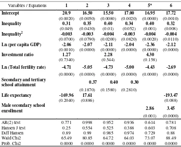
28
Table 4. Redistribution vs. Inequality (b): segmented sample
Highly developed tax system
Variables / Equations 1 2 3 4
Redistribution -242.07 -162.11 -186.85 -182.29
(0.0003) (0.0072) (0.0048) (0.0025)
Dummy: Latin America 11.18 7.01
(0.0000) (0.0003)
Dummy: Asia 6.64
(0.0968)
Dummy: Household vs.
Individual 9.09 7.31
(0.0001) (0.0001)
Dummy: Gross or net
income -8.43 -5.06
(0.0002) (0.009)
Dummy: Income or
expenditure data -10.28 -7.67
(0.0002) (0.0006)
Intercepts 50.6, 51.7, 55.5, 49.5
45.1, 44.7, 48.4, 42.2
55.0, 56.8, 61.2, 56.5
50.2, 51.4, 56.1, 50.7
Number of Observations 38, 36, 44, 31 38, 36, 44, 31 20, 21, 24, 18 20, 21, 24, 18
R-squared 0.17, 0.06, 0.05, 0.13
0.21, 0.22, 0.12, 0.58
0.39, 0.48, 0.56, 0.68
0.50, 0.59, 0.54, 0.81
Variables identical to table 2
The next step, after demonstrating the negative relationship between redistribution and
inequality, was to test for the non linearity of the relationship between inequality and
growth in order to validate the proposed model. Table 5 reports the results of an initial
set of estimations via the Seemingly Unrelated Regression methodology where the Gini and its square value as well as other explanatory variables16 were included.
Equation 1 initially demonstrates (in line with most studies based on the Deininger and
Squire, 1996 complete dataset) the fact that the majority of the observations and
correspondence between inequality and growth data of the complete sample are located
on the negative range of the relationship. When including in this first estimation the
Gini coefficient together with life expectancy and three religion dummies it was evident
the negative overall relationship between inequality and growth. In this general case, a
5% decrease in the Gini coefficient of would raise the GDP per capita growth rate in
1.3%.
16
29
Equations 2 to 4 test for the non linearity between inequality and growth by
incorporating the square value of the Gini coefficient. The estimation results show that
the coefficients for both variables are significant, especially when introducing the Latin
American dummy.
The sign of the Gini coefficient is positive while the square Gini is negative,
demonstrating the fact that at low levels of inequality (lower than the ORI) the
relationship is positive, and at high levels of inequality, the relationship is negative.
The level of inequality at which the relationship changes, is at an approximated Gini
value of .39. At this level, the economy grows higher than at any other level. These
results verify the existence of an optimal rate of inequality, at which the economy is
released from any distortion from either high inequality or high taxation/redistribution
(and low inequality).
As expected, the reciprocal of life expectancy at birth as well as the religion dummies
(Catholic, Protestant and Muslim) show a negative effect on growth rates. Equation 4
includes the price level of investment as explanatory variable as a measure of price
distortions in the economy, this variable appeared to account for some of the effects
previously captured by the religion dummies and the reciprocal of life expectancy,
[image:30.595.116.481.539.756.2]while increasing the effects of both Gini and Gini2.
Table 5. Inequality and growth relationship (SUR estimation)
Variables / Equations 1 2 3 4 5
Gini -0.022 0.10 0.13 0.15 -0.03
(0.036) (0.109) (0.05) (0.0200) (0.0283)
Gini2 -0.001 -0.0016 -0.002
(0.049) (0.026) (0.012)
Latin American dummy -0.67 -0.8
(0.0448) (0.0169)
1/life expectancy at birth -194.12 -182.61 -189.87 -162.41 -140.56
(0.0000) (0.0000) (0.0000) (0.0000) (0.0017)
Catholic dummy -1.67 -1.59 -1.14 -0.97
(0.0000) (0.0000) (0.009) (0.0289)
Protestant dummy -2.45 -2.27 -2.16 -1.71
(0.0000) (0.0001) (0.0001) (0.0027)
Muslim dummy -1.03 -1.05 -1.06 -1.02
(0.0164) (0.0139) (0.012) (0.0141)
PPPI -0.007
(0.0039)
Gini x Redistribution 0.39
30
Intercepts 8.4, 6.7, 6.8, 7.1 5.6, 3.9, 4.0, 4.3 5.0, 3.2, 3.4, 3.7 4.6, 2.9, 3.06, 3.4 5.9, 4.2, 4.5, 4.8
Number of Observations 63, 69, 76, 92
63, 69, 76, 92
63, 69, 76, 92
59, 67, 74, 91
42, 39, 51, 69
R-squared 0.3, 0.20, 0.25, 0.01 0.3, 0.18, 0.24, 0.07 0.27, 0.17, 0.27, 0.08 0.33, 0.18, 0.30, 0.08 0.15, 0.1, 0.1, 0.13
Independent variable is average GDP growth for each 10 year period (70s,80s, 90s, and 00s). Estimation made by the Seemingly Unrelated Regression technique. Explanatory variables are: Gini, Square Gini, Latin American dummy, the reciprocal of life expectancy at birth, three religion dummies that equals one if the majority of the population profess either Catholic, Protestant or Muslim religion, and the price level of investment (PPPI). Intercepts from equations 1-4 are significant at the 1 and 5 percent, the remaining are significant to the 1 percent.
Equation 5 adds an interaction term between inequality measured by the Gini coefficient
and redistribution in order to further validate the non-linearity of the relationship
between inequality and growth. The results confirmed that at low levels of redistribution
the relationship between inequality and growth is negative (because inequality will be
high), but as redistribution increases, this relationship will attenuate and will eventually
turn positive when reaching a level of redistribution equivalent to approximately 11% of
GDP.
An additional set of systems were estimated via 3SLS based on Barro (2008) in which
economic indicators were included as explanatory variables. The potential endogeneity
of some of the independent variables is addressed with a set of instruments that comply
with the requirements of being correlated with the explanatory variables and not being
correlated with the error term (see notes on Table 6). The three stage least squares
(3SLS) estimator, proposed by Zellner and Theil (1962), considers the specific error
term as random and provides asymptotical efficient estimations that come from
exploiting nonzero cross equation covariation.17
The systems incorporate typical explanatory variables employed in standard growth
models such as the log of per capita GDP and the investment ratio. These level variables
resulted in all cases as expected, the first one with a negative coefficient that confirm
conditional convergence and the second one with a positive and significant one
depicting the contribution of investment to GDP growth.
17
31
The log of the total fertility rate shows negative effects on growth, although statistically
significant to the 5% in most cases. The reciprocal of life expectancy at birth turned to
be barely significant in the linear estimation (Equations 1 and 2), but when testing for
non-linearity (Equations 3 to 6), it became statistically insignificant. The political
instability variable, though surprisingly positive, has almost null effects on growth
while total school attainment for secondary and tertiary education turned to be
statistically insignificant.
Equations 1 and 2 of Table 6 test for the overall effects of inequality over growth. The
results are consistent with the ones in Equation 1 of Table 5. In this case, lowering
inequality from a Gini level of .40 to .39 would increase the GDP per capita growth rate
in 1.73%. This result and the fact that the average Gini for the four decades is .43
demonstrate once again the fact that the sample as a whole is located predominantly in
the negative spectrum of the relationship between inequality and growth. (see
Appendixes 1 and 2)
Equations 3 to 6 report the results of testing for the non linearity of the relationship
between inequality and growth. This was verified initially by including the square value
of the Gini coefficient. In all cases, a positive sign for the Gini coefficient and a
negative one for its square value were found. Appendix 3 depicts the kinked non-linear
relationship between inequality and growth computed with the coefficients of the
regressions.
As in the SUR estimation, is was found that at a Gini of .39 is the breakpoint where the
growth rate is maximized and where the sign of the relationship changes Equation 4
incorporates a dummy that accounts for the level of development of the tax system, as
well as a dummy for Latin America in order to control for the effects of a tendency for
some Latin American countries of having high inequality combined with high growth
rates. Both variables turned to be statistically insignificant, nevertheless, when the price
level of investment is included in Equation 5, the Latin American dummy turns
statistically significant with a negative sign. Price distortions seem to capture whatever
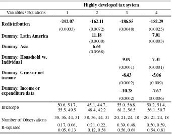
32
Lastly, Equation 7 includes the interaction term between inequality and growth (Gini x
Redistribution). Once again it was verified the fact that as redistribution increases, the
relationship turns from being initially negative to positive, in this case, when reaching a
level of redistribution equivalent to approximately 5.8% of GDP. This value is
considerably lower than the one obtained in the SUR estimation, perhaps because
Equation 5 of Table 5 did not include economic variables which could capture a portion
[image:33.595.85.525.253.642.2]of the effects of redistribution on inequality and ultimately on growth.
Table 6. Inequality and growth relationship (3SLS estimation)
Variables / Equations 1 2 3 4 5 6 7*
Gini -0.04 -0.02 0.22 0.23 0.23 0.022 -0.06
(0.0341 (0.0502) (0.0076) (0.0045) (0.0044) (0.0074) (0.003)
Gini2 -0.002 -0.003 -0.003 -0.003
(0.003) (0.0022) (0.002) (0.0023)
Log(per capita GDP) -1.56 -1.48 -1.19 -1.39 -1.002 -1.11 -1.68
(0.0000 (0.0000) (0.0000) (0.0000) (0.0001) (0.0000) (0.0000)
Log(Total fertility rate) -1.67 -1.51 -1.61 -1.59 -1.27 -1.5 -2.07
(0.0253 (0.0153) (0.0151) (0.0179) (0.0515) (0.0212) (0.0062)
1 / life expectancy at
birth -166.11 -153.32 -89.58 -88.4 -108.5 -70.76
(0.0736) (0.0183) (0.1618) (0.2087) (0.1086) (0.2889)
Investment ratio 7.89 4.46 6.12 8.52 5.78 6.63 9.37
(0.0023) (0.0419) (0.0038) (0.0001) (0.0043) (0.0013) (0.0017)
Political instability
variable 0.0086 0.01 0.007
(0.0015) (0.0005) (0.0092)
PPPI (Price level of
investment) 0.001 -0.005 -0.002
(0.3748) (0.1993) (0.5218)
Secondary and tertiary
school attainment 0.12
(0.3748)
Dummy: developed tax
revenue system 0.19
(0.4231)
Dummy: Latin America -0.28 -0.64
(0.3241) (0.0181)
Gini x Redistribution 0.52
(0.006)
Intercepts 21.1,19.6, 19.8,19.8 19.8,18.3, 18.1,18.0 11.4,10.1, 9.9,10.1 12.2,10.8, 10.9,10.9 9.8,8.5, 8.4,8.5 10.4,9.1, 9.0,9.1 18.34,18. 6, 18.76
Number of Observations 28,53,47, 49 46,61,66, 82 46,62,69, 87 45,58,65, 82 46,62,69, 87 46,62,69,
87 44,39,40
R-squared 0.25,0.47, 0.57,0.05 0.38,0.03 0.21,0.4, 0.25,0.32, 0.3,0.1 0.23,0.41, 0.31,0.14 0.27,0.3, 0.33,0.1 0.28,0.31, 0.29,0.11 0.53,0.53, 0.16