http://dx.doi.org/10.4236/me.2016.79095
Researches on the Inter-Provincial
R&D Innovation Efficiency for
Chinese High-Tech Industry
Kexin Liu
School of Economics, Jinan University, Guangzhou, China
Received 24 June 2016; accepted 28 July 2016; published 1 August 2016
Copyright © 2016 by author and Scientific Research Publishing Inc.
This work is licensed under the Creative Commons Attribution International License (CC BY). http://creativecommons.org/licenses/by/4.0/
Abstract
The characteristics of Chinese economic area are distinct, and the development status of the inter- provincial high-tech industry is significantly different. As Chinese high-tech industry is acting an increasingly important role in pushing the economic development, it is necessary to evaluate the inter-provincial R&D innovation efficiency for high-tech industry. This text, using the DEA Ap-proach with Double Frontiers, made comparison for the evaluation unit with the “optimized” and “worst” decision-making unit respectively. Therefore it carried out measurement for the inter- provincial optimistic efficiency and pessimistic efficiency for Chinese high-tech industry, and sug-gested the comprehensive results with the geometric average efficiency. The research results showed that there were great differences among the R&D innovation efficiencies for Chinese high- tech industry among 26 provinces and municipalities. There is no need for the high-tech industry to blossom everywhere. It, based on the economic development and efficiency status, should be strengthened in Beijing, Tianjin, Guangdong, Chongqing and Jiangsu, etc.
Keywords
High-Tech Industry, R&D Innovation Efficiency, Inter-Province, DEA Approach with Double Frontiers
1. Foreword
High-tech industry, with the general characteristics such as the high knowledge intensity, high technology inten-sity and high intelligence inteninten-sity, etc., is the most active industry in innovation among the economic activities. High-tech mainly refers to the information technology, bio-engineering and new materials, etc. Under the condi-tion in 2013, when the world economy maintained the “weak growth”, the Chinese high-tech industry had still shown a strong power with the main business income increasing from the 4.9714 trillion Yuan in 2007 to over 11 trillion in 2013, an uplifted rate of 10% in 2013, and with the products export amount increasing from 287,000 million USD in 2007 to 558,200 million USD in 2013. China now has become the biggest export coun-try for the high-tech products in the world, with the total export-import volume for the high-tech induscoun-try taking 29.3% of the total amounts of the commodities import and export in 2013. Looking from the perspective of the trade mode, however, the export for the Chinese high-tech industry takes the main means of processing trade, but the trade for the technology level and R&D abilities still takes a low proportion. 84% of the R&D expendi-tures in 2013 were used for the experimental development while the fundamental research and applied research took 4.7% and 10.7% respectively, maintaining great differences with the developed countries in the allocation proportion. In China where the R&D resources are not sufficient, the inputs-outputs efficiency is quite impor-tant.
In the past, the measurement of the R&D innovation efficiency for the high-tech industry mainly employed the DEA model to evaluate the effective decision-making unit. And the major existing problem was the multiple subjective factors. Besides, for the traditional DEA model, the evaluation unit was only compared with the “op-timized” decision-making unit to obtain the “op“op-timized” result, therefore the analysis was one-sided. However, this text employs the DEA Approach with Double Frontiers, which makes comparison between the evaluation unit with the “optimized” and “worst” decision-making unit to get a comprehensive result. As a result, compared with the traditional DEA method, the DEA Approach with Double Frontiers has added the perspectives for comparison and comparatively reduced the subjective factors, which makes the results more comprehensive.
This text, through measuring the inter-provincial comparative efficiency of the Chinese high-tech industry, aims to have a deeper understanding of the current inputs-outputs efficiency status of the Chinese high-tech in-dustry, providing certain references to the allocation of the R&D resources in the industry. On the other hand, it will help the provinces and municipalities to get a brief idea of the improvement space for the efficiency and avoid the waste of resources.
2. Literature Review
The quick development of the high-tech industry in recent years and its feature of possessing high innovation ability have attracted the attention of some scholars. Scholars used different methods and point of research on high technology industry efficiency. Study results show that China's innovation efficiency is low. For example, Zhu Youwei and Xu Kangning (2006) [1] have employed the stochastic frontier production function (SFPF) to measure the relative R&D innovation efficiency for the various sub-industries in the Chinese high-tech industry and obtained the conclusion of a comprehensive low R&D innovation efficiency. Guan Jiancheng and Chen Kaihua (2009) [2], with the data envelopment method, carried out analysis on the technological innovation effi-ciency for the Chinese high-tech industry. The results also showed that the comprehensive technological innova-tion efficiency for the Chinese high-tech industry is relatively low as well. Liu Chuan (2012) [3] performed measurement on the high-tech innovation efficiency for provinces and municipalities of China with the three-phased DEA method. And the results showed R&D innovation efficiency for Chinese high-tech industry is also on the low side. Huang Guibao (2014) [4], with the data envelopment method and the spatial econometrics, performed measurement on the innovation efficiency for the high-tech industry in provinces and municipalities of China. The results show that the innovation efficiency is in increasing in general, but the R&D and scale effi-ciency is in declination.
3. Research Methods
DEA model, firstly established by Charnes, Cooper and Rhodes (1978) [9], is a non-parameter method to eva-luate the comparative efficiency of a group of decision-making units. The DEA model in the traditional way is making a comparison of the relative efficiency with the “optimized” unit. In other words, the largest degree that the inputs can be reduced with equal proportion under the unchanged outputs of that year, therefore the results obtained are called as optimistic efficiency. In the inputs-oriented model, the optimistic efficiency values ob-tained are less than or equal to 1. As it is the comparison of the comparative efficiency of the decision-making units, there must exist the evaluation unit whose efficiency value exactly equals to 1. The decision-making unit with a value equals to 1 is called as effective unit. It is located on the effective frontier and represented by OE. The decision-making unit with the efficiency value of less than 1 is with relatively void efficiency, which is represented by ON. It can be noted clearly that the optimistic efficiency of the OE decision-making unit is better than that of ON.
Parkan and Wang (2000) [5] proposed to measure the comparative efficiency of the decision-making unit from the pessimistic perspective of view. In the inputs-oriented model, the pessimistic model represents the largest degree that the inputs can be increased with equal proportion under the unchanged outputs. In other words, it is the efficiency value obtained by comparing with the “worst” decision-making unit. This efficiency is called as pessimistic efficiency. All the pessimistic efficiencies equal to 1 at least. If the efficiency value of the decision-making unit equals to 1, it means that it is on the void frontier and in the void state. It is represented by PI. If the efficiency value is larger than 1, it means it is on the non-void state and it is represented by PN. It should be noted that the PN in the non-void state does not necessarily equals to the OE in effective state. And it is usually thought that the pessimistic efficiency of the decision-making unit of PI is worse than that of PN.
The effective frontier and the void frontier constitute the double frontiers. The geometric average efficiency proposed by Wang and Chin (2007) [10] has soundly integrated the optimistic and pessimistic efficiency for the analysis of the results.
3.1. Optimistic Model
CCR model, as the first data envelopment model, was proposed by Charnes, Cooper and Rhodes (1978) [9]. The basic principle of the CCR model is to measure the comparative efficiency through the outputs-inputs proportion. Assume we need to measure the comparative efficiency for n decision-making units, and there are m kinds of inputs and q kinds of outputs for each decision-making unit. xij represents the inputs volume for the jth deci-sion-making unit on the ith kind of inputs while yrj represents the outputs volume for the jth decision-making unit on the rth kind of outputs, in which i=1, 2,,m, r=1, 2,,q. Use vi (i=1, 2,,m) and ur (r=1, 2,,q) respectively to represent the weight between the inputs and outputs. Then the outputs-inputs ratio for the evaluation unit j can be represented as:
1 1 q r rj r j m i ij i u y v x θ = = =
∑
∑
(1)
In the model (1), the appropriate weight can always be found to make θj ≤1. To add limitation conditions to model (1), and the model is as follows:
1
1
1
1
max
. . 1, 1, ,
, 0, 1, , ; 1, , .
q r ro r o m i io i q r rj r j m i ij i r i u y v x u y
s t j n
v x
u v r q i m
Thereinto, DUMO is the evaluation unit on-going while vi and ur are the decision-making variables of the model. The inherent meaning of the CCR model is as following: Under the condition of making the effi-ciency values of all the decision-making units equal to or less than 1, maximize the effieffi-ciency value of the eva-luated unit. Therefore the weight determined at this time is the optimized one. That is to say the CCR model is making a conservative estimation for the void condition of the decision-making unit evaluated. CCR model is with constant returns to scale. It means if u* and v* is the optimized solution for model (2), then for any t > 0,
*
tu and tv* is also the optimized solution for the model. The model (2) is not only the non-linear programmed, but also there are infinite optimized solutions. So it is necessary to covert model (2) into the equivalent linear programming model. The method is proposed by Charnes and Cooper (1962) [11] as follows:
1
1 1
1
max
. . 0, 1, ,
1
, 0, 1, , ; 1, , .
q
o r ro
r
q m
r rj i ij
r i m i io i r i u y
s t u y v x j n
v x
u v r q i m
θ = = = = = − ≤ = = ≥ = =
∑
∑
∑
∑
(3)
Its dual model is:
1
1
min
. .
0
1, , ; 1, , , 1, , .
n
j ij io j
n
j rj ro j
s t x x
y y
r q i m j n
θ λ θ λ λ = = ≤ ≥ ≥ = = =
∑
∑
(4)The optimized solution for the objective function of model (4) is θ*. What the 1−θ* represents is the larg-est degree that the inputs can be cut under the current technological level and under the condition that the
O
DUM evaluated doesn’t reduce the outputs level. The smaller the θ* is, the larger the range for the inputs can be cut and the lower the efficiency is. If θ =* 1, it means that the DUMO is located on the effective fron-tier. Under the condition of not reducing the outputs, there is no space for equal-proportioned declination for kinds of inputs. It is in the effective technology state OE. If it is less than 1, it means the decision-making unit is in the void state ON. In other words, under the condition of not reducing the outputs, the kinds of inputs are al-lowed to decline with the proportion of
(
1−θ*)
.3.2. Pessimistic Model
The pessimistic model means the largest degree that the inputs can be increased under the condition of not in-creasing the outputs level. That is the comparative efficiency compared with the “worst” decision-making unit. The pessimistic efficiency model is proposed by Parkan and Wang (2000) [5]:
1
1
1
1
min
. . 1, 1, ,
, 0, 1, , ; 1, , .
q r ro r o m i io i q r rj r j m i ij i r i u y v x u y
s t j n
v x
u v r q i m
Being the same to the optimistic one, the pessimistic efficiency model is also non-linear. And there are also infinite optimized weight solutions for it. Therefore it shall also rely on the conversion method proposed by Charnes and Cooper (1962) [11] to convert the non-linear programming model to the linear model:
1
1 1
1
min
. . 0, 1, ,
1
, 0, 1, , ; 1, , .
q
o r ro
r
q m
r rj i ij
r i m i io i r i u y
s t u y v x j n
v x
u v r q i m
ϕ = = = = = − ≥ = = ≥ = =
∑
∑
∑
∑
(6)Its dual model is:
1
1 max
. .
0
1, , ; 1, , , 1, , .
n
j ij io j
n
j rj ro j
s t x x
y y
r q i m j n
ϕ λ ϕ λ λ = = ≥ ≤ ≥ = = =
∑
∑
(7)
The optimized solution for the objective function of model (7) is ϕ*. And the ϕ*−1 means the largest de-gree that its inputs can be increased under the current technological level and under the condition where the
O
DUM evaluated doesn’t increase the outputs level. If ϕ* =1, it means O
DUM is on the void frontier. Un-der the condition of not increasing the outputs, there is no equal-proportioned increasing space for its kinds of inputs. That is PI. If ϕ* >1, the decision-making unit is on the non-void technology state PN. That is to say under the condition of not increasing the outputs, its kinds of inputs can be increased with the proportion of (ϕ*−1). The larger the ϕ* is. The larger the range that the inputs can be increased, the higher the efficiency is.
3.3. Geometric Average Efficiency
The optimistic efficiency model and the pessimistic efficiency model are measuring the efficiency for the deci-sion-making unit from different perspectives of view. And the ranking results of the efficiencies are generally different. The different measuring results reflect different information. Looking independently, each kind of these is only considering the comparison from one perspective. To obtain a more comprehensive analysis, it is necessary to integrate the two kinds of results. Wang and Chin (2007) [10] propose the following geometric av-erage efficiency model:
* * *
γ = θ ϕ⋅
(8)
In the model, θ* is the efficiency value for the optimistic model of the evaluation unit, while ϕ* is the ef-ficiency value for the pessimistic model and γ* is the geometric average efficiency value. As the geometric average efficiency includes the optimistic and pessimistic efficiencies, the geometric average efficiency of each of decision-making unit can be treated as the efficiency measured by the DEA Approach with Double Frontiers.
4. Empirical Analysis
outputs while the sales income for the new products represents the economic outputs index for the R&D innova-tion. In conclusion, the measurement of the R&D innovation efficiency for the high-tech industry includes two inputs indexes and two outputs indexes. In the DEA model, the more the number of the decision-making units is, the more obvious the distinction degree and the more objective the results are. If there are few decision-making units, there will be number of effective units. Cooper (2007) [14] proposed a rough rule for the number of deci-sion-making units and indexes. In other words, the number of the decideci-sion-making units n is larger than max{3 × (m + q), m × q}, in which m is the number of inputs indexes and q is the number of outputs indexes. Accord-ing to this rule, it is reasonable for this text to select the number of decision-makAccord-ing unit and number of inputs and outputs indexes for analysis.
This text employed the 6-year data of the 2000, 2005, 2010-2013, and all the data comes from the Statistical Yearbook for Chinese High-Tech Industry of the Year 2014. Data is selected from 2000, 2005, 2010-2013 based mainly on the following reasons: 1) Through the DEA Approach with the Double Frontiers data and according to years of operation, data which is not continuous will not affect the empirical results; 2) Based on Five-Year Plan of the Chinese government; 3) Consider the availability of data. For all these reasons, this article chooses 2000, 2005, 2010-2013 data. With MATLAB (2012) software, it carried out the optimistic and pessimistic efficiency measurement for the model data, and the geometric average efficiency was obtained from the excel calculation.
4.1. Optimistic Model Results Analysis
[image:6.595.91.538.341.701.2]It can be drawn through Table 1 that Tianjin, Beijing, Guangdong and Yunnan have a high optimistic efficiency.
Table 1. Optimistic efficiency status of Chinese high-tech industry inter-provincially.
Region 2000 2005 2010 2011 2012 2013 Average value
Beijing 0.77 0.87 1.00 1.00 1.00 1.00 0.94
Tianjin 1.00 1.00 1.00 0.94 1.00 1.00 0.99
Hebei 0.22 0.10 0.32 0.33 0.55 0.44 0.33
Shanxi 0.18 0.33 0.95 0.44 0.39 0.34 0.44
Liaoning 0.31 0.20 0.33 0.50 0.36 0.44 0.36
Jilin 0.13 0.20 0.61 0.38 0.82 0.88 0.50
Heilongjiang 0.39 0.19 0.16 0.20 0.27 0.18 0.23
Shanghai 0.52 0.48 0.54 0.65 0.57 0.46 0.54
Jiangsu 0.68 0.53 0.51 0.77 0.73 0.61 0.64
Zhejiang 0.58 0.45 0.48 0.52 0.57 0.50 0.52
Anhui 0.07 0.24 0.29 0.37 0.70 0.73 0.40
Fujian 1.00 0.66 0.56 0.58 0.65 0.46 0.65
Jiangxi 0.07 0.11 0.32 0.27 0.45 0.48 0.28
Shandong 0.51 0.37 0.49 0.63 0.47 0.37 0.47
He’nan 0.44 0.20 0.43 0.38 0.43 1.00 0.48
Hubei 0.09 0.10 0.60 0.40 0.40 0.38 0.33
Hu’nan 0.22 0.21 0.57 0.54 0.57 0.57 0.45
Guangdong 0.39 0.33 0.89 0.92 1.00 1.00 0.76
Guangxi 0.21 0.16 0.27 0.30 0.63 0.69 0.38
Chongqing 0.14 0.25 0.70 1.00 0.66 0.51 0.54
Sichuan 0.85 0.22 0.20 0.32 0.64 0.52 0.46
Guizhou 0.13 0.22 0.36 1.00 0.82 0.60 0.52
Yunnan 1.00 1.00 1.00 0.59 0.69 1.00 0.88
Shanxi 0.05 0.12 0.21 0.23 0.23 0.26 0.18
Gansu 0.26 0.10 0.16 0.33 0.36 0.32 0.26
Ningxia 0.28 0.17 0.60 0.41 0.34 0.31 0.35
Among which Beijing and Tianjin have a sound development basis and large inputs in the high-tech industries and they have kept the national-leading status for a long time. Beijing’s optimistic efficiency from 2010 to 2013 is OE. For Tianjin, only the year 2011 of 0.94 is not on the effective frontier in the six years. Guangdong prov-ince ranks last in the optimistic efficiency in 2000. However, with the transition of the economic structure, Shenzhen has undergone a fast development together with other innovation cities. So, it was listed on the effec-tive frontier together with Beijing and Tianjin from 2010.Then we can assume that the Guangdong Province has achieved certain success in the transition and the R&D inputs for the high-tech industry has have been fully utilized. Yunan Province, which takes tourism as the pillar industry, has a relatively weak basis for high-tech industry. Both the number of R&D personnel and the internal expenditure for R&D maintain a relatively low level throughout the country, so do the number of effective invention patents and the outputs of new products sales income.
Fujian, Zhejiang, Shanghai, Jiangsu and Chongqing maintain a relatively high optimistic efficiency. Among which there is generally no big fluctuations in the optimistic efficiency for Zhejiang, Shanghai and Jiangsu, while the optimistic efficiency for Fujian takes a declining rank inter-provincially. In other words, compared with the provinces on the optimistic frontier, Fujian obtains a year-on-year declining outputs for the same inputs. Therefore, Fujian province should improve the utilization rate of the inputs and avoid the waste of resources. With the advance of the development of western regions, Chongqing, as the core city in the southwest China, it has increasing inputs for its high-tech industry by the year. And its optimistic efficiency ranks among the top ones in the provinces.
Heilongjiang, Shaanxi, Gansu and Ningxia have relatively low optimistic efficiencies, among which Heilong-jiang displays an obviously declining tendency in optimistic efficiency. Compared to Jilin, the inputs of R&D personnel and the expenditure of Heilongjiang Province are higher. But its output is far lagged behind. As lo-cated in the western regions, Shaanxi, Gansu and Ningxia are with an underdeveloped economy, and maintain relatively low absolute amount and relative amount for the inputs of high-tech industry.
Generally speaking, there are vast distributions of optimistic efficiency values. But most of them are distri-buted between 0.4 - 0.7. And there are 13 provinces and municipalities with values in this region. The average value of the optimistic efficiency value is 0.495 and there are 11 provinces and municipalities with values higher than this. The provinces and municipalities with a higher optimistic efficiency are the direct-controlled munici-palities or distributed in the economically developed zones such as the coastal areas. While for the provinces and municipalities in the underdeveloped regions such as the western regions and the northeast regions, they main-tain a relatively low optimistic efficiency. The optimistic efficiencies of the R&D innovation for Chinese high-tech industry have obvious regional differences.
4.2. Pessimistic Model Results Analysis
It can be drawn from Table 2 that Guangdong Province has the highest average value of pessimistic efficiency, followed by Beijing and Tianjin. The pessimistic efficiency of all the three provinces and municipalities are dis-playing a rising tendency.
Shanghai, Jiangsu, Chongqing and Yunnan have relatively high pessimistic efficiencies. And they are quite stable with no great fluctuations.
Heilongjiang, Shaanxi, Gansu and Ningxia maintain relatively low pessimistic efficiencies. Thereinto, the pessimistic efficiency of Heilongjiang Province displays an obviously declining tendency and it is on the non- effective frontier for four successive years from 2010 to 2013.
Generally speaking, there are vast distributions of pessimistic efficiency values. Its average value is 1.949. And there are 14 provinces and municipalities with values under this. The provinces and municipalities with high pessimistic efficiencies are the directly-controlled municipalities or those located on the developed areas as the coastal areas. While for the provinces and municipalities in the underdeveloped areas as the western regions and the northeast China, they maintain a relatively low pessimistic efficiency. There is no much difference be-tween the inter-provincial ranking of pessimistic efficiency and the ranking of pessimistic efficiency. The pes-simistic efficiencies of the R&D innovation for Chinese high-tech industry maintain obvious regional differenc-es. And this regional difference is generally in coincidence with the optimistic efficiency.
4.3. Geometric Average Efficiency Analysis
op-Table 2. Pessimistic efficiency status of Chinese high-tech industry inter-provincially.
Region 2000 2005 2010 2011 2012 2013 Average value
Beijing 1.85 2.43 6.06 3.64 3.82 4.17 3.66
Tianjin 1.37 1.88 3.71 2.36 3.80 2.98 2.68
Hebei 1.02 1.00 1.18 1.24 1.72 1.89 1.34
Shanxi 2.58 3.16 2.16 1.52 1.04 1.00 1.91
Liaoning 2.72 1.75 1.10 1.00 1.10 1.33 1.50
Jilin 2.17 1.33 1.78 1.37 1.73 2.58 1.83
Heilongjiang 1.95 1.37 1.00 1.00 1.00 1.00 1.22
Shanghai 3.58 1.16 3.49 2.45 2.29 2.19 2.53
Jiangsu 2.48 1.68 1.72 1.78 2.78 2.19 2.11
Zhejiang 1.14 1.10 2.51 2.15 2.08 2.08 1.84
Anhui 1.00 2.28 1.42 1.17 2.44 3.68 2.00
Fujian 1.00 2.68 1.42 1.14 1.92 1.57 1.62
Jiangxi 1.00 1.07 1.12 1.00 1.36 1.71 1.21
Shandong 2.98 1.38 2.11 1.44 1.74 1.53 1.86
Henan 2.00 1.93 1.29 1.00 1.00 1.00 1.37
Hubei 1.00 1.00 1.15 1.97 1.64 1.98 1.46
Hunan 2.16 1.79 2.75 1.97 2.06 1.17 1.98
Guangdong 3.92 2.14 5.45 4.43 3.63 5.20 4.13
Guangxi 1.16 1.54 2.15 1.42 2.54 3.06 1.98
Chongqing 2.90 2.30 2.32 2.14 2.02 2.79 2.41
Sichuan 2.94 1.24 1.01 1.26 2.58 2.66 1.95
Guizhou 1.70 2.15 1.98 3.76 1.49 1.03 2.02
Yunnan 2.23 2.49 3.38 2.62 1.59 3.30 2.60
Shaanxi 1.00 1.21 1.09 1.00 1.00 1.10 1.07
Gansu 1.04 1.00 1.00 1.22 1.46 1.36 1.18
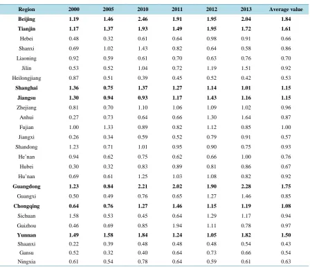
[image:8.595.73.539.98.468.2]timistic and pessimistic model analysis results on the evaluation of the overall efficiency. It can be drawn from
Table 3 that Beijing has the largest average value of geometric average efficiency, which is 1.84. The next is Guangdong, which is 1.75. Shannxi, among the 26 provinces and municipalities, maintains the minimum aver-age value of geometric averaver-age efficiency, which is 0.43. It is over four times less compared with the value of Beijing. The provinces and municipalities with an average value of geometric average efficiency of above 1.00 include Beijing, Tianjin, Shanghai, Jiangsu, Chongqing and Yunnan. There are 19 provinces and municipalities with values lower than this standard. The average value of the average value of the geometric average efficiency is 0.95. Its standard deviation is 0.37 and the median is 0.92. That is to say, the values of the geometric average efficiency are with a relatively high concentration and small dispersion. Generally speaking, the geometric av-erage efficiency is for Chinese high-tech industry in 26 provinces and municipalities are all around the avav-erage value, except the high values of Beijing, Tianjin and Guangdong.
4.4. Efficiency Distribution Diagram Analysis
The efficiency diagram is divided into four regions by the average-value line, which is the upper left, lower left, upper right and lower right. In the upper right region, there are 8 provinces and municipalities whose optimistic efficiency and pessimistic efficiency are higher than the average value. Thereinto, Guangdong, Beijing, Tianjin and Yunnan maintain relatively high optimistic efficiencies and pessimistic efficiencies, followed by Shanghai,
Table 3. Geometric average efficiency status of Chinese high-tech industry inter-provincially.
Region 2000 2005 2010 2011 2012 2013 Average value
Beijing 1.19 1.46 2.46 1.91 1.95 2.04 1.84
Tianjin 1.17 1.37 1.93 1.49 1.95 1.72 1.61
Hebei 0.48 0.32 0.61 0.64 0.98 0.91 0.66
Shanxi 0.69 1.02 1.43 0.82 0.64 0.58 0.86
Liaoning 0.92 0.59 0.61 0.70 0.63 0.76 0.70
Jilin 0.53 0.52 1.04 0.72 1.19 1.51 0.92
Heilongjiang 0.87 0.51 0.39 0.45 0.52 0.42 0.53
Shanghai 1.36 0.75 1.37 1.27 1.14 1.01 1.15
Jiangsu 1.30 0.94 0.93 1.17 1.43 1.16 1.15
Zhejiang 0.81 0.70 1.10 1.06 1.09 1.02 0.96
Anhui 0.27 0.73 0.64 0.66 1.30 1.64 0.87
Fujian 1.00 1.33 0.89 0.82 1.12 0.85 1.00
Jiangxi 0.26 0.34 0.59 0.52 0.79 0.91 0.57
Shandong 1.23 0.71 1.01 0.95 0.90 0.75 0.93
He’nan 0.94 0.62 0.75 0.62 0.66 1.00 0.76
Hubei 0.30 0.32 0.83 0.89 0.81 0.86 0.67
Hu’nan 0.69 0.61 1.25 1.03 1.08 0.82 0.92
Guangdong 1.23 0.84 2.21 2.02 1.90 2.28 1.75
Guangxi 0.50 0.49 0.76 0.65 1.27 1.46 0.85
Chongqing 0.64 0.76 1.27 1.46 1.15 1.19 1.08
Sichuan 1.58 0.53 0.45 0.64 1.29 1.17 0.94
Guizhou 0.46 0.69 0.85 1.94 1.11 0.78 0.97
Yunnan 1.49 1.58 1.84 1.24 1.05 1.82 1.50
Shaanxi 0.22 0.39 0.48 0.48 0.48 0.54 0.43
Gansu 0.52 0.32 0.40 0.64 0.73 0.66 0.54
Ningxia 0.61 0.54 0.78 0.64 0.59 0.61 0.63
Chongqing and Jiangsu. The 8 provinces and municipalities are located in the developed area, except Yunnan and Guizhou. In the upper left region, the optimistic values are lower than the average value and the pessimistic values are higher or equal to the average value. Guangxi, Anhui, Hu’nan and Sichuan are included in this area. There is no many differences in the pessimistic efficiencies for these four provinces and municipalities. Howev-er, for the optimistic efficiency, Sichuan is higher than Hu’nan. Hu’nan is higher than Anhui. Anhui is higher than Guangxi. This sequence is consistent with the economic development status. In the lower right region, all the optimistic efficiencies are higher than the average value and the pessimistic efficiencies are lower than the average value. Zhejiang, Jilin and Fujian are included in this area. In other words, under the condition of un-changed outputs, the equal-proportioned declination degree for the inputs is low. The same to the equal- propor-tioned increase. Therefore, for this region, the increase of inputs would bring a large rise of the outputs. The lower left region covers 12 provinces and municipalities-almost half of the sum. Both the optimistic efficiencies and the pessimistic efficiencies in this region are lower than the average level. The values of the provinces and municipalities in this region are far lower than below the average value line, except Shanxi and Shandong, where their values are slightly lower than the average.
To sum up, according to the efficiency diagram, the 26 provinces and municipalities of China can be catego-rized into three levels. The first level covers Guangdong, Beijing, Tianjin and Yunnan. The second level covers 14 provinces, which are around the average value line. The third level covers 8 provinces and municipalities, whose optimistic and pessimistic efficiencies are far below the average value line. In conclusion, there are ob-vious regional differences for inter-provincial R&D innovation efficiency for Chinese high-tech industry and the efficiencies are generally low.
4.5. The R&D Innovation Efficiency Status Analysis for Eight Economic Zones
It can be drawn from Table 4 that the Northern Coastal Economic Zone, the Southern Coastal Economic Zone and the Northeast Coastal Economic Zone maintain obviously higher R&D innovation efficiency than other economic zones, among which the Southern Coastal Economic Zone is the highest in the R&D innovation effi-ciency. Within the Southern Coastal Economic Zone, Guangdong is higher than Fujian Province in the R&D innovation efficiency. It can be observed that Guangdong Province is in a leading position for the R&D innova-tion efficiency for the high-tech industry in China. There is no much difference lying among the three provinces and municipalities in the Eastern Coastal Economic Zone. Their R&D innovation efficiency levels are in general coincidence. Within the Northern Coastal Economic Zone, the R&D innovation efficiencies of Beijing and Tianjin are obviously higher than Hebei and Shandong. The R&D innovation efficiency in the Yangtze River Mid-stream Economic Zone is in an obvious rising tendency. Benefited from the Development of the Western Region, the Southwest Economic Zone maintains a high level of R&D innovation efficiency within the inland area. The Northeast Economic Zone and the Yellow-river Midstream Economic Zone are ranking last among the eight economic zones for the R&D innovation efficiency. Located in the inland area, these two economic zones are lagged behind in economic and innovation level. In conclusion, the R&D innovation efficiency in the coastal area is relatively high and that in the inland area is generally low.
5. Conclusions and Suggestions
This article carried out comprehensive analysis on the inter-provincial optimistic efficiency, the pessimistic effi-ciency and geometric average effieffi-ciency for Chinese high-tech industry with the DEA Approach with Double Frontiers. And the following conclusions have been drawn:
Table 4. The R&D innovation efficiency for the eight economic zones.
Zone 2000 2005 2010 2011 2012 2013
TheNorthern Coastal Economic Zone
Beijing 1.19 1.46 2.46 1.91 1.95 2.04
Tianjin 1.17 1.37 1.93 1.49 1.95 1.72
Hebei 0.48 0.32 0.61 0.64 0.98 0.91
Shandong 1.23 0.71 1.01 0.95 0.90 0.75
Average value 1.02 0.96 1.50 1.25 1.44 1.36
TheSouthern Coastal Economic Zone
Fujian 1.00 1.33 0.89 0.82 1.12 0.85
Guangdong 1.23 0.84 2.21 2.02 1.90 2.28
Average value 1.12 1.09 1.55 1.42 1.51 1.56
The Eastern Coastal Economic Zone
Jiangsu 1.30 0.94 0.93 1.17 1.43 1.16
Zhejiang 0.81 0.70 1.10 1.06 1.09 1.02
Shanghai 1.36 0.75 1.37 1.27 1.14 1.01
Average value 1.16 0.80 1.13 1.16 1.22 1.06
The Yellow-river Midstream Economic
Zone
Shaanxi 0.22 0.39 0.48 0.48 0.48 0.54
He’nan 0.94 0.62 0.75 0.62 0.66 1.00
Shanxi 0.69 1.02 1.43 0.82 0.64 0.58
Average value 0.62 0.67 0.89 0.64 0.59 0.71
The Northwest Economic Zone
Gansu 0.52 0.32 0.40 0.64 0.73 0.66
Ningxia 0.61 0.54 0.78 0.64 0.59 0.61
Average value 0.57 0.54 0.59 0.64 0.66 0.64
The Northeast Economic Zone
Liaoning 0.92 0.59 0.61 0.70 0.63 0.76
Jilin 0.53 0.52 1.04 0.72 1.19 1.51
Heilongjiang 0.87 0.51 0.39 0.45 0.52 0.42
Average value 0.77 0.54 0.68 0.63 0.78 0.90
The Southwest Economic Zone
Sichuan 1.58 0.53 0.45 0.64 1.29 1.17
Chongqing 0.64 0.76 1.27 1.46 1.15 1.19
Guizhou 0.46 0.69 0.85 1.94 1.11 0.78
Guangxi 0.50 0.49 0.76 0.65 1.27 1.46
Yunnan 1.49 1.58 1.84 1.24 1.05 1.82
Average value 0.93 0.81 1.03 1.19 1.17 1.28
The Yangtze River Mid-stream Economic
Zone
Hubei 0.30 0.32 0.83 0.89 0.81 0.86
Hu’nan 0.69 0.61 1.25 1.03 1.08 0.82
Anhui 0.27 0.73 0.64 0.66 1.30 1.64
Jiangxi 0.26 0.34 0.59 0.52 0.79 0.91
Average value 0.38 0.50 0.83 0.78 1.00 1.06
Note: In consideration for the obtaining status of the data, Inner Mongolia, Hainan, Qinghai, Tibet, Sinkiang, Hong Kong, Macao and Tai-wan are not included in this table.
Based on the conclusions above, this article makes the following suggestions. Firstly, China has to deepen the scientific management system and lift the conversion abilities for the scientific and technological fruit as well as reduce the waste of the R&D inputs. Secondly, when the government is making relevant policies, it can add reasonable R&D inputs and optimize the resources allocation combining with the relative R&D innovation effi-ciency of the sub-industry and the current scale. Thirdly, China has to enhance the inputs for the high-tech in-dustry in Guangdong, Beijing and Tianjin. And the regions mentioned above shall take multiple measures to promote the development of the high-tech industry. Part of regions can be gradually transformed the economic structure to allow a stable and quick development of the high-tech industry. For example, the high-tech industry in Shenzhen has obtained some fruit.
References
[1] Zhu, Y.W. and Xu, K.N. (2006) Empirical Researches on the R&D Innovation Efficiency for the China High-Tech In-dustry. Chinese Industrial Economy, No. 11, 38-45
[2] Guan, J.C. and Chen, K.H. (2009) The Measurement for the Technological Innovation for China High-Tech Industry.
Quantity Economy Technology Economic Researches, No. 10, 19 -33
[3] Liu, C. (2012) Researches on the R&D Innovation Efficiency for China High-Tech Industry. Industrial Technology Economy, No. 12, 19-25
[4] Gui, H.B. (2014) Economic Econometrics Analysis on the Innovation Efficiency and the Influencing Factors for China High-Tech Industry. Economic Geography, No. 6, 100-107.
[5] Parkan, C. and Wang, Y.M. (2000) Worst Efficiency Analysis Based on Inefficient Production Frontier. Information Sciences, 175, 20-29.
[6] Entani, T., Maeda, Y. and Tanaka, H. (2002) Dual Models of Interval DEA and Its Extension to Interval Data. Euro-pean Journal of Operational Research, 136, 32-45.http://dx.doi.org/10.1016/S0377-2217(01)00055-8
[7] Wang, Y.M. and Chin, K.S. (2009) A New Approach for the Selection of Advanced Manufacturing Technologies DEA with Double Frontiers. International Journal of Production Research, 47, 6663-6679.
http://dx.doi.org/10.1080/00207540802314845
[8] Wang, Y.M. and Lan, Y.-X. (2011) Measuring Malmquist Productivity Index: A New Approach Based on Double Frontiers Data Envelopment Analysis. Mathematical and Computer Modelling, 54, 2760-2771.
http://dx.doi.org/10.1016/j.mcm.2011.06.064
[9] Charnes, A., Cooper, W.W. and Rhodes, E. (1978) Measuring the Efficiency of Decision Making Units. European Journal of Operational Research, 2, 429-444.http://dx.doi.org/10.1016/0377-2217(78)90138-8
[10] Wang, Y.M., Chin, K.S. and Yang, J.B. (2007) Measuring the Performances of Decision Making Units Using Geome-tric Average Efficiency. Journal of the Operational Research Society, 58, 929-937.
http://dx.doi.org/10.1057/palgrave.jors.2602205
[11] Charnes, A., and Cooper, W.W. (1962) Programming with Linear Fractional Functionals. Naval Research Logistics Quarterly, 9, 181-186.http://dx.doi.org/10.1002/nav.3800090303
[12] Sharma, S. and Thomas, V.J. (2008) Inter-Country R&D Efficiency Analysis: Application of Data Envelopment Anal-ysis. Scientometrics, 76, 483-501.http://dx.doi.org/10.1007/s11192-007-1896-4
[13] Bai, J.H., Jiang, K.S. and Li, J. (2009) Comprehensive Evaluation and Analysis on the Innovation Efficiency of the Regional Innovation System in China. Management Review, No. 9, 3-9.
Submit or recommend next manuscript to SCIRP and we will provide best service for you:
Accepting pre-submission inquiries through Email, Facebook, LinkedIn, Twitter, etc. A wide selection of journals (inclusive of 9 subjects, more than 200 journals) Providing 24-hour high-quality service
User-friendly online submission system Fair and swift peer-review system
Efficient typesetting and proofreading procedure
Display of the result of downloads and visits, as well as the number of cited articles Maximum dissemination of your research work