Subjectivity in Application of the Principle of Maximum Entropy

http://dx.doi.org/10.4236/ojs.2013.36A001

Subjectivity in Application of the Principle of Maximum

Entropy

Jan Peter Hessling

Measurement Technology, SP Technical Research Institute, Borås, Sweden Email: [email protected]

Received September 24, 2013; revised October 24, 2013; accepted November 1, 2013

Copyright © 2013 Jan Peter Hessling. This is an open access article distributed under the Creative Commons Attribution License, which permits unrestricted use, distribution, and reproduction in any medium, provided the original work is properly cited. In accor- dance of the Creative Commons Attribution License all Copyrights © 2013 are reserved for SCIRP and the owner of the intellectual property Jan Peter Hessling. All Copyright © 2013 are guarded by law and by SCIRP as a guardian.

ABSTRACT

Complete prior statistical information is currently required in the majority of statistical evaluations of complex models. The principle of maximum entropy is often utilized in this context to fill in the missing pieces of available information and is normally claimed to be fair and objective. A rarely discussed aspect is that it relies upon testable information,

which is never known but estimated, i.e. results from processing of raw data. The subjective choice of this processing

strongly affects the result. Less conventional posterior completion of information is equally accurate but is computa- tionally superior to prior, as much less information enters the analysis. Our recently proposed methods of lean determi- nistic sampling are examples of very few approaches that actively promote the use of minimal incomplete prior infor- mation. The inherited subjective character of maximum entropy distributions and the often critical implications of prior and posterior completion of information are here discussed and illustrated, from a novel perspective of consistency, rationality, computational efficiency and realism.

Keywords: Maximum; Entropy; Bayes; Monte Carlo; Uncertainty; Covariance; Deterministic; Sampling; Testable;

Information; Model; Calculation; Simulation

1. Introduction

The principle of maximum entropy (PME) can be uti- lized to determine a probability density distribution func- tion (pdf) from incomplete statistical information. The approach is not limited to determination of prior pdfs in Bayesian estimation, even though that is a common ap- plication. It is rather a general recipe how to make known but incomplete statistical information complete with the most ‘fair’ or the weakest possible hypotheses. As such it fits very well into our practice of statistics, where the lack of complete information is the rule rather than the exception. For instance, knowing only the mean and the variance of an uncertain parameter PME results in a normal distribution [1]. The known information must be well defined in a statistical sense, i.e. be formulated in

terms of statistical expectations f

 

 of functions

 

f  of the considered random quantity . For in- stance, f

 

  yields the mean and f



q

 

k with estimators [2] fˆ to give testable informa-

tion f

 

fˆ



 





 

 

produces the moment around the mean. Their expectations can be estimated from any set of observations

-th

q

k

    [3].

kurtosis etc. Various statistical moments around the mean are tested, as if they were terms of a Taylor series. The functions gq 



 



q are indeed the

order monomial related to a Taylor expansion around the mean. The expectation

-th q

q

g will contribute to the non- linear displacement h

 

 h







, or scent [5] of

order, of the model . For any other statistic like e.g. covariance, no such simple direct relation holds [6]. Another line of reasoning might be that the mean des- cribes the location of the distribution, the second moment the width, the third the lowest order asymmetry, while the fourth is the lowest order shape indicator etc. We might subjectively claim that these properties (location- width-asymmetry-shape) provide a hierarchy of testable information. This does not imply that the moments themselves drop in magnitude or relevance, with their order. On the contrary, the linearly scaled even moments

-th

q h

 

1 2 2 2

q

q q

M  g  usually increase with the order .

In the limit q ,

q

  M₂q maxk k , where k are

the observations of .

Given a set of observations it is not evident how they should be processed to provide testable information of the highest possible quality, i.e. with minimal residual

uncertainty. For instance, which moments gq should

be estimated with a quality (variance of estimator) that usually decrease with the order ? As will be shown, the selection will directly influence the PME distribution function. It is also not evident why PME should be re- stricted to prior application, as usually practiced. Post- erior utilization might in fact simplify the analysis great- ly. After all, PME is a general method with no explicit reference to what the distribution describes, the input or the output of the analysis.

q

2. Method of Maximum Entropy

For a continuous sample space , the entropy [4] func- tional to be maximized in the method of maximum en- tropy is given by the Lebesgue integral,



 

log



 



d .

S p  p  



 

_

(1.1)

The bar-symbol restricts the integration over dis- tinguishable outcomes     . That accounts for

our possible ignorance1 _{of not distinguishing distinct}

outcomes. As there is an obvious contradiction of being aware of ignorance, it is better translated into irrelevance (for our stated problem). The integration over  can be extended to , by locally measuring the relative density

of



 with the Lebesgue measure m

 

 ,

 

d m  d . Consistency requires transformation invariance [1] of the probability dP in the interval

, d

    . That is, p

 

d  p

 

 d , giving the

substitution p

 

  p

   

 m  . This invariance is equivalent of requiring independence [3] of dP

 

 on the subjectively chosen parameterization. In fact, that constraint provides a direct method of determining the Lebesgue measure: If  , m

 

 d m

 

 d . For instance, ignorance to change of units correspond to the transformation  

 

, where  describes the conversion factor between different units. It yields

 

d

 

d m

  

d



m





d m   m        or

 

1 m   .

Utilizing m

 

 the integral in Equation (1.1) is con- verted into a Riemann integral,

 

log p

 

_{ }

m d .



S p  



 



 



, 0,1

 

_

_

, 2, ,

i N

(1.2)

The optimization is subject to all known testable information i   ,

 

   

d p

 

f_i

 

d ,

i  fi  



p  fi   



   (1.3) 

0 1, 0 1.

f    (1.4) The functions k will for convenience be denoted

test functions. The mandatory zeroth constraint ₀ f



(Equation (1.4)) is the normalization condition. As point- ed out [3], for discrete sample spaces and no degeneracy ( ), there is a general expression for the maxi- mum of Equation (1.1) in terms of a partition function

const m=

Z . It can be generalized to non-constant measures

 

m  , and continuous distributions using calculus of

variations [7],

 

_e i1i i

f

Z m

  

d .

  







_

(1.5)

The Lagrange multipliers of optimization are implic- itly given by the testable information,

log 0, 1, 2, , ,



i i

Z  i  N





  

 (1.6)

0 log .Z

  (1.7)

The maximum entropy pdf is then given by,

 

 

_e 0  _,

N i i i

f

p m

 

      _{. (1.8)}

2.1. Testable Information

The PME solution (Equation (1.8)) does not specify the test functions . They are of major importance though since the solution is directly expressed in them. As stated in the introduction there is a convention of setting ₁

,

k

f k1

f , f2



 



2 etc. That is a habit, not

a prescription. The choice of test functions must con- sequently be considered to be at our free disposal.

1_{Remark: “Ignorance” will here refer to the aspect of counting}

dependent on the explicit form of fk. Also, the in-

formation contained in the observation set

 

k is to a

variable degree transferred to the estimate of fk

 

 .

For instance, if f

 

 

q q

all observations are equally weighted, but if f g

   

,

, ,

q

g    q     (1.9)

the exponent determines how much different obser- vations contribute. In the asymptotic limit , the observation with the largest deviation is much more important than any other (which only contributes to the estimate of the mean). A lot of information is obviously disregarded. The estimator covariance will accordingly be large. Nevertheless, in many situations the range [6]

q

q 

 

1 2 max

k

2

limk g k   k   is of much larger

interest than any other information. The confidence in- terval is a more general statistic allowing for sample spaces without bound. From the perspective of objec- tivity, it thus appears difficult to prescribe any specific set f kk, 1, 2, , N

N

, or even their number (N). Clearly,

the larger amount of data or independent information that is available, the larger is allowed without resulting in unacceptable estimator quality, as expressed with its bias and covariance.

To illustrate how subjectivity enters in practice, assume we have gathered a set of prior observations

 

k of a phenomenological constant  contained in a

computer model. To calibrate the model [8], i.e. de-

termine the optimal values of its parameters and their uncertainties ( being one of them) from observations, Bayesian estimation is applied. That requires complete prior information, i.e. knowledge of the prior pdf p

 

 .

Applying PME starting from



k



, test functions



k

f 



must be selected. With the choice of f1g1

 

 ,

q

 

2

f g  , the partition function will according to

Equation (1.5) read,

 

Z m  _e1 1g   2gq  _d_.

 

_

Since we are not aware of any ignorance, we set . The condition Equation (1.6) on

 

1

m   g1

 

 im-

plies,

 

1 2

0 1 e    q

Z _   d .



_

A fair amount of subjective pragmatism now suggests to be limited to even numbers and the support

q  to

extend to the whole real axis, since that allows us to determine 1 with ease. The symmetry of the integrand

then implies 10. If 0 is prohibited, 10.

The current assignment then translates into an appro- ximation of the support  as well as the factor

 

1

e     1

of p

 

 . The remaining Lagrange multi- plier 2 is obtained by re-scaling,

 

2 1

2

e qd q e dtq _,

Z 



_     



_  t

 

2 2

log 1 _.

q

Z g

q



 



  



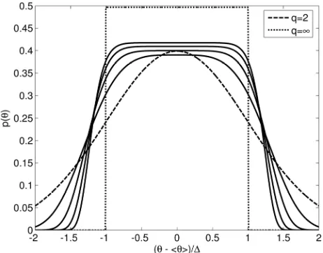
The resulting pdf,

 

 

_{ }

1

e gq q, q

q

p       g  , (1.10)

where  describes the q-th order “width” of the pdf

 

p  , is for different displayed in Figure 1. Clearly,

the PME pdf is to a significant extent controlled by our subjective choice of test function, i.e. . The result

varies between normal

q

q



q2



and uniform



q 



.

More generally, with the understanding of the depend- ence on the test functions fi (Equation (1.8)), almost

any PME pdf can be generated. It is only a matter of formulating the question (selecting fi) to obtain the ans-

wer



p

 





on virtually any desired form.

2.2. Quality of Estimation

In practice, a testable piece of information i is esti-

mated from raw observations with quality depending on the test function fi. The maximum entropy pdf p

 



can be directly formulated in our observations

 

 k _,

using a specific estimator of the moment around the mean. An obvious estimator is given by,

-th

q

       

1 1

1

ˆq q n k n k q_,

k k

S B

n

 

 



 _ 

 





 (1.11)

where  q is an unknown constant which hopefully

[image:3.595.306.537.67.181.2] [image:3.595.308.539.471.652.2]

B

can be selected to eliminate the bias, e.g.  2 ₁



₁



B  n .

To express the bias of in terms of expand and calculate its expectation over observations

  ˆq

S B q ,

 

 

_ k

,

    0 0 1

0 2 0 ! 1 ˆ _. ! j n j j

q k _n

k

q q k k

n

j

k q _j

j

S B n

n k             _ _   







q (1.12) On the other hand,

 

_{ }

 





0 1 ! . ! ! q k q q k q q k k q S

k q k

         



(1.13)

Clearly, the number of terms of  q

S is much less

than for ˆ q

S for q3. Elimination of bias by  q

B

proper selection of requires proportionality be- tween  q

S and Sˆ q . That cannot in general be achieved since one of them have much more terms than the other. Thus, no scaling of ˆ q

S can make it uni- versally unbiased. Evaluating the first two coefficients of the expansion in Equation (1.12),

   



       











1 1 1 2 1 0 ˆ

! 1 1

1

! !

q q q q q q

q q k q q q q q k

S B n c q c

q

c c q

k q k n n

                  _ _    _{ }     



 . q (1.14) Surprisingly, these two terms satisfies the proportio- nality required to eliminate the bias. Bias can thus be eliminated by rescaling up to , but not for (see estimation of kurtosis in [9]). This suggests the normalization,

3

q q4

 









1 1 2 0

! 1 ₁ 1

! ! k q q q k q

B n q

k q k n n

             _ _ _    _ _    



.      (1.15) While  2 ₁



₁



B  n , B 4 1



n 4 6 n23 n3





. Clearly, bears little resemblance to the

conventional form  4

B



1 nz of , where is the number of degrees of freedom.

 2

B z

After failing to obtain an unbiased estimator of the moment around an unknown mean, we may lower the ambition by assuming the mean

-th

q

 is known. The corresponding estimator reads,

   



1

ˆ_{q q} n q_,

k k

T B  











(1.16)

This is a considerably simpler situation for which the normalization  q 1

B 

 

ˆ var

 

ˆ _.

ˆ

M M

M

  (1.17)

The least possible variance of any unbiased estimator of

 q

S gq

 

 is given by the Cramer-Rao lower

bound [2] _ q _{, evaluated in Appendix A,}

 

 

 _. 2 q q S n

    q

(1.18)

Since _ q _{increases with , it is indeed more}

difficult to determine higher order moments accurately on an absolute scale, with any estimator. The efficiency

q

 of our specific estimator measures its relative quality,

 q

ˆ T      

 





 





1 !! 1, ˆ _{2 2 1 !! 1 !!}

q q

q

q q

T q q

     

 _    _ (1.19)

where m!!

 

m m2



m4



1

  , is even and the precision

 

ˆq q

T



1

is evaluated in Appendix B. For an

efficient [2] estimator,  . A low value of  means

that the potential for improvement of our estimator is large. Since _ q _{decreases rapidly with , also}

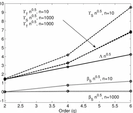
becomes worse on a relative scale as increases. Nev- ertheless, the actual precision may or may not be satisfactory. The performance of the estimators is illustrated and compared to the Cramer-Rao lower bound in Figure 2, by evaluating their relative variation

q Tˆq

ˆ, S T q  ˆ 

and bias  numerically with multiple Monte Carlo ensembles.

To conclude, the determination of the PME pdf in- volved several subjective choices of processing the ob- servations. The shape was here restricted by using mono- mial test functions

 

g_q . The order was limited to

be even, to simplify the calculation of the integrals. Likewise, an infinite symmetric sample space

q

 was assigned. The difficulty of estimating various statistical moments around the mean increases rapidly with the order. If there are not more than a few samples it is in most cases impossible to reliably estimate any other moments than the first and the second. The application of PME thus relied upon rational selection rather than ob- jective deduction.

2.3. Prior vs Posterior Application of PME The PME constructs complete pdfs from incomplete testable information. It can be applied to the input (PME prior), or the output (PME post(-erior)) of the analysis. As no restriction or preference is stated in PME, both alternatives deserves to be considered and evaluated for efficiency and accuracy. The default method of lineari- zation (LIN) [10] as well as the unscented Kalman filter (UKF) [11,12] and deterministic sampling (DS) [6] n makes the estimator unbiased

[image:5.595.59.287.83.277.2]

Figure 2. The relative precision and (dashed,

Equation (1.17)) for the estimators

S



  ˆq

T



S (Equation (1.11)) and (Equation (1.16)), respectively, compared to the Cramer-Rao lower bound (solid, Equation (1.18)), for

(connected by lines for clarity) and  

ˆq

T 2,4,6



q n10, 1000

samples. The relative bias  q of Sˆ q (dotted, given by Equation (1.15)) is also shown. The calculations were made for randomly generated samples of a normal distributed variable, equally split into ensembles of

samples. Scaling with account for the main dependences on the number of samples (Equation (1.18)).

 q

B

7 10

n n0.5

n

in general propagate statistics like covariance which later can be expanded to information related to entire pdfs, e.g. confidence intervals. That is, LIN, UKF, and DS pro- motes PME post. Monte Carlo simulations [13] or ran- dom sampling (RS) must start with complete statistical information to determine its random generator, i.e. RS

requires PME prior.

An elementary example illustrates the principal dif- ferences between PME prior and PME post. Assume it is of interest to calculate the 95% confidence interval



h ha, b



of an uncertain model h







, dependent on one

parameter . Let the model uncertainty [8] be given by the mean  0 and the variance

 

 2 1. PME prior determines the input pdf f

 

 to be normal

distributed. Repeated generation of RS ensembles esti- mates their variation as function of their size: To achieve a standard deviation of the input confidence in- terval

95%



 a, b



for  of about , no less than

around randomly generated samples of

5%

3000  are

required. In RS, the model is evaluated for all these samples of  and



,



1, 2,a b h h

, 

is found by evaluating the results , ordering them, and extracting the 95% percentiles. The known statistics

 

 

k ,

h  k 3000

0

  and

 

 2 1 can however be encoded

exactly in no more than two(!) deterministic (calculated

with a rule) samples . Assuming the model is close to linear-in-parameters, the model vari- ance is mainly determined by the parameter variance, here represented by the parameter ensemble . In DS, the model variance is then with the argument of consistency given by the second moment around the mean of the model ensemble , i.e.

 1 _1,  2 ₁

    

 

 

k ,

h  

(2) (1)_,



1, 2 k

 





2

 

 

 1

_{ }

2

 

 2 ₂

h 2 h h h 2 h 

   _   _ .

Applying PME post to the result h and

 

h 2 implies that the resulting pdf is normal distributed, ana- logously to the input pdf in RS. That implies a coverage factor of k1.96 resulting in a confidence interval,





 

 

 

_{ }

 

 





2 1 2 2

,

1,1 . 2

a b

h h

h h

h k

    

  

(1.20)

For estimating confidence intervals, PME does not in fact need to be utilized at all. By using another DS tech- nique of ours, sampling on confidence boundaries [5], the desired interval can be found directly as,





 

2

 

2

,

, .

a b

h h

h  k  h  k 

    

_{ }  _{ }  _

   

 

(1.21)

Consistency in evaluating confidence intervals of models here lead to the related concept of confidence boundaries in parameter space. For multivariate models with non-linear dependencies on parameters, both these results needs to be properly generalized [5,6]. Propa- gating a PME prior probability density function thus

typically require several thousands of model samples [13,14] or complex algorithms [15]. The number of

model samples propagated with DS for final completion with PME post can be as few as for para- meters and increases with the known statistical infor- mation, the complexity of the model and acceptable accuracy of evaluation [16].

1 

n n

given by a finite Taylor expansion can be exactly cal- culated with stratified DS [16]. Similarly, the confidence interval of any model

 



T

h    





T

,



of any number (n) of parameters can be evaluated exactly [5], where

are constants,



1 2 n

     



T

1 2 n

      all parameters, and 

 

x is any non-linear monotonic function. For comparison, we are not aware of any general analytic method to pro- pagate a univariate pdf determined by PME prior through any non-linear model. In this case, RS is a numerical method that yield arbitrarily small errors, but at very high computational cost. For “genuinely” multivariate prob- lems RS seizes to be accurate. Multivariate refers to non- trivial finite dependencies of any order, as required for optimal modeling [16]. As far as we know, higher order dependencies (beyond second moments and not normal distributions) can only be implemented in RS by ex- cluding samples. Exceptionally dense sampling is then required to accurately represent sampling density over

the entire -dimensional sampling domain. Neverthe- less, it is straight-forward to represent any arbitrary mixed moment in stratified DS [16]. The difficulty is just that the more requirements, the more samples are re- quired. If not enough samples can be afforded it is possible to find the best approximating ensemble where different requirements are given different weights of im- portance. There are thus several reasons (as exemplified here) for PME post methods to not only be superior to PME prior approaches in efficiency, but also accuracy. The lean set of known input information in PME post is much simpler to analyze or propagate through any model than the complete information in PME prior.

n

With these observations, the traditional preference to prior instead of posterior completion of information with PME appears biased and strongly subjective. It is highly questionable if PME post methods like DS [6,11,16,17] can be claimed less accurate than state-of-the-art RS relying upon PME prior per se. As both practice sta- tistical sampling once defined by Enrico Fermi [18], they

are fully comparable. The choice is critical for complex models, as the low efficiency of RS easily render an impossible numerical task. Indeed, that is the main cur- rent obstacle for wide utilization of uncertainty quan- tification with RS.

Bayesian estimation is formulated for PME prior. The combination of the maximum likelihood function and the prior distribution makes Bayes approach superior to traditional approaches limited to the former. In practice though, two functions (PME prior) or two discrete sets of

statistics (PME post) derived from observations are fused. Indeed, the common assumption of Gaussian noise and PME prior derived from the mean and covariance results in combination of covariance matrices (numbers) and not pdfs [8]. A non-trivial posterior distribution function

requires non-Gaussian and/or correlated noise and uti- lization of no less than an infinite set of testable reliable

information in the PME prior. If not so, Bayes estimation can without any loss of accuracy and relevance be made with PME post instead of PME prior, e.g. with DS instead of RS [8].

PME post (DS) makes it evident that results seldom are unique, while PME prior (RS) conceals ambiguities in more or less dubious or blind assignments in the problem set up. The indefiniteness of the result is an unavoidable consequence of starting with incomplete information, not the analysis. For PME post analyses (DS) this can easily be illustrated, for instance using different ensembles [6]. It is considerably more difficult for PME prior analyses (RS) due to their prohibiting numerical complexity. The contradictory consequence is that PME prior generally are considered more credible than PME post analyses, even if the latter are more honest and real- istic as their flaws easily can be illustrated.

2.4. Towards Consistency and Rationality

The PME test functions should be selected according to the evaluation of the model, its behavior, and the quality of estimating the corresponding testable information. If we are interested in propagating the covariance of a signal processing model [6], we should consequently use a distribution which has been tested for representation of covariance. That is a consistent rather than an objective

choice. Objectivity is an impossible target—selecting any

method is a subjective choice. Our ignorance of p

 

 is rather reflecting relevance in perspective of our pri- mary interest, or consistency throughout the analysis. It appears that consistency summarizes the goals of objec- tivity as well as our ignorance [1,3,4] and emphasizes the context. In contrast to objectivity, consistency expresses a relativity that can indeed be achieved in many situa- tions, as well as measured, questioned and criticized.

The ubiquitous sparsity of statistical information in virtually all practical problems needs to be seriously addressed. If the realism of two approaches are com- parable but their efficiency distinctively different, the choice should be based on rationality rather than con-

minute fraction of the statistical information used in PME prior.

3. Conclusions

The character of maximum entropy (PME) distribution functions has been discussed. There are two principal innovations of our study. The PME solutions can to some extent be controlled by how primary data is processed. The prevailing preference for applying PME to the input (prior) and not the output (posterior) of statistical analy- ses is difficult to justify, as the their accuracy is compa- rable but the latter is computationally superior. The choice appears governed by the method of analysis. Hence, subjectivity enters into the processing of data as well how the analysis is made.

A non-trivial selection enters when observations are processed into testable information. A simple example illustrated common subjective choices, giving different results for identical observations.

Redirecting the focus from the treatment of known in- formation to the targeted evaluation of the analysis em- phasizes consistency, rather than objectivity. When con-

sistency is indecisive, rationality or efficiency of the

analysis provides obvious guidance. PME can be applied to find prior as well as posterior distributions. Its uncon- ventional posterior application deserves to be seriously considered, as the analysis involves much less statistical information and is correspondingly more effective, than the prior. Consistency and rationality thus fundamentally questions the prevailing method of completing statistical information prior to the analysis, as in e.g. Monte Carlo simulations.

Maximal consistency and rationality are indeed pri- mary goals of all our proposed methods of deterministic sampling. For complex models, such lean and custom- ized approaches are often required to obtain any measure of modeling quality at all (within acceptable computa- tional time). Without assessment of quality, any (model- ing) result is of no value. These aspects are thus of para- mount importance to our society where complex calcula- tions (technical, physical, econometrical etc.) are rapidly increasing due to the fast development of computers.

REFERENCES

[1] D. S. Sivia and J. Skilling, “Data Analysis—A Bayesian Tutorial,” Oxford University Press, Oxford, 2006. [2] S. M. Kay, “Fundamentals of Statistical Signal

Process-ing, Estimation Theory,” Volume 1, Prentice Hall, Upper Saddle River, 1993.

[3] E. T. Jaynes, “Information Theory and Statistical Me- chanics,” The Physical Review, Vol. 106, No. 4, 1957, pp. 620-630. http://dx.doi.org/10.1103/PhysRev.106.620 [4] C. E. Shannon, “A Mathematical Theory of

Communica-tion,” The Bell System Technical Journal, Vol. 27, No. 3, 1948, pp. 379-423.

[5] J. P. Hessling and T. Svensson, “Propagation of Uncer- tainty by Sampling on Confidence Boundaries,” Interna-tional Journal for Uncertainty Quantification, Vol. 3, No. 5, 2013, pp. 421-444.

[6] J. P. Hessling, “Deterministic Sampling for Propagating Model Covariance,” SIAM/ASA Journal on Uncertainty Quantification, Vol. 1, No. 1, 2013, pp. 297-318.

[7] G. M. Ewing, “Calculus of Variations with Applications,” Dover, New York, 1985.

[8] J. P. Hessling, “Identification of Complex Models,” in Review, 2013.

[9] L. Råde and B. Westergren, “Mathematics Handbook,” 2 Edition, Studentlitteratur, Lund, 1990.

[10] ISO GUM, “Guide to the Expression of Uncertainty in Measurement,” Technical Report, International Organisa- tion for Standardisation, Geneva, 1995.

[11] S. Julier and J. Uhlmann, “Unscented Filtering and Non- linear Estimation,” Proceedings IEEE, Vol. 92, No. 3, 2004, pp. 401-422.

[12] S. Julier, J. Uhlmann and H. Durrant-Whyte, “A New Approach for Filtering Non-Linear Systems,” American Control Conference, Seattle, 21-23 June 1995, pp. 1628- 1632.

[13] R. Y. Rubenstein and D. P. Kroese, “Simulation and the Monte Carlo Method,” 2 Edition, John Wiley & Sons Inc., New York, 2007.

[14] J. C. Helton and F. J. Davis, “Latin Hypercube Sampling and the Propagation of Uncertainty in Analyses of Com- plex Systems,” Reliability Engineering and System Safety, Vol. 81, No. 1, 2003, pp. 23-69.

http://dx.doi.org/10.1016/S0951-8320(03)00058-9 [15] T. Lovett, “Polynomial Chaos Simulation of Analog and

Mixed-Signal Systems: Theory, Modeling Method, Ap- plication,” Lambert Academic Publishing, Saarbrücken, 2006.

[16] J. P. Hessling, “Stratified Deterministic Sampling of Mul- tivariate Statistics,” in Preparation, 2013.

[17] J. P. Hessling, “Deterministic Sampling for Quantifica- tion of Modeling Uncertainty of Signals,” In: F. P. G. Márquez and N. Zaman, Eds., Digital Filters and Signal Processing, INTECH, Rijeka, 2012.

Appendix A Cramer-Rao Lower Bounds of

Statistical Moments of a Normal Distributed

Variable

Assume a random variable  with zero mean is normal distributed, N



0,



 q q

M 



1



q3



. By integrating by parts it can be shown that , where

is the semi-factorial function. The probability distribution function for



5

q



1 !!

q



1



q1 !!



 q



can then be expressed in (q)

M ,

 







_{ }





_{ }



2 2

2

1 !! 1 !!

0, exp .

2

q q

q

q _q

q q

p N

M _M

  

 _{  } 

    

 _ _

 

 _{ } 

 



(1.22) For independent observations

 

, the likelihood function is given by,

n k ,k1, 2, , n

 

 









 





 





 

 

_

_

 

2 2

2 1

2 2 2

1

1 !! 1 !!

1 _exp

2π ₂

1 !! 1 !!

exp .

2

q k

q n

q

k q

q _q

k

q n q

n k q

q _q

k

p M

q q

M _M

q q

M _M











 _{  }

   

  

 

 _{ } 

 

 _{  } 



     

   

 

  _{  } 





 



(1.23)

Cramer-Rao lower bound ([2]) now states that for any estimator ˆ q

M of M q ,  

 

ˆ 1

 

var q ,

M F  (1.24)

where F

 

 is the Fisher information matrix (scalar for one parameter),

 

 

 





 

 

2

2 2

2

ln ₂

.

q k

q

p M _n

F

q M

 





  

 (1.25)

The expected precision (Equation (1.17)) of the estimator



 q

M hence satisfies,

 

 

 

ˆ var

. 2

q

q

M _q

n M

   (1.26)

Appendix B Variance of Estimator of

Statistical Moments around Given Mean

An estimator of the q-th statistical moment

 q

_

_

q

M    of  around a known mean  from a set of n independent observations

 

k is

given by,

 

_

1

ˆ q n q_,

k k

M B  











(1.27)

where the normalization constant B is chose to minimize

its bias ˆ q  

M M q . Since  is a known constant it is trivially found that B1 n eliminates all bias, for all values of q. Its variance is found to be,

 

 

     

  2 2

2 2

ˆ

var .

q q

q q q M M

M M M

n n

 

 

 

 _{ }   

(1.28) An explicitly value can be found for a normal dis- tributed parameter, N



0,



. Then, by recursively

integrating by parts it is found that , where

 q q

_

_{1 !!}

_

M  q



q1 !!

 

 q1



q3



q5



1 is the semi- factorial function, giving

 

 

_ˆ



2 1 !!

 

1 !!



var q q q q .

M

n

   