STUDIES ON IMPROVING TEXTURE SEGMENTATION PERFORMANCE USING GENERALIZED GAUSSIAN MIXTURE MODEL INTEGRATING DCT AND LBP

(1)

ISSN: 1992-8645 www.jatit.org E-ISSN: 1817-3195

322

IMPLEMENTATION OF SENSORLESS CONTROL OF AN

INDUCTION MOTOR ON FPGA

USING XILINX SYSTEM GENERATOR

1

SGHAIER NARJESS, 1TRABELSI RAMZI, 1MIMOUNI MED FAOUZI 1

The National Engineering School of Monastir, Ibn El jazzar City, 5019, Monastir,

E-mail: [email protected], [email protected]

,

[email protected]

ABSTRACT

In this paper, we will presented a deterministic observation approach , nonlinear applied to the Induction Motor: this is a sliding mode observer. Indeed, this paper will serve to emphasize the importance of the order without sensor to increase the profitability of our machine. Our sliding mode observer will be applied to the field oriented vector control then to the sliding mode control. The contribution of this paper is the design of sensorless control using XSG order to be implanted on the FPGA.

Keywords: Induction motor, FPGA, Sensorless Control, Sliding mode observer, XSG

1. INTRODUCTION

In the literature, the majority of developed control laws require speed control. In fact, it requires a mechanical sensor namely a tachometer dynamo or an incremental encoder. But unfortunately some applications need other techniques for reconstitution of speed because of the variables that are not accessible to measurement are usually the magnetic variables and this is mainly due to economic reasons and reliability of measurement. The most used technique is the use of observers. An observer is usually installed on a calculating to reconstruct or to estimate in real time the state of a system, from the available measures of the inputs of the system variables and of a priori knowledge of the model. The role of an observer to monitor the dynamics of the state as a basic information on the system. To increase the robustness of the control and improve performance, we will use a sliding mode observer for the reconstitution of the speed and other inaccessible variables to the extent such that the rotor flux. To highlight the performance and benefits related to the use observers. We proposed in this paper to implement this observer for two commands without mechanical sensors.

The contribution of this paper is the use of the graphical environment XSG is a new tool in the field of machine control and allows electrical engineers to quickly design control algorithms that are typically too difficult to be programmed and requires great knowledge in the fields of electronics and the major advantage of this tool is to avoid the

painful programming and away from the usual tools such as Labview and VHDL without forgetting that this tool allows viewing of all signals before FPGA implementation.

The contribution At first we will start with the vector control with sensors observing of the rotor flux. Then we will focus on the sliding mode control without mechanical speed sensor. Then we implemented the two control laws: the vector control and the sliding mode control on FPGA board using X_ilinxS_ystemG_enerator_{(XSG). At the}

end of this paper a comparative study will be made between results obtained using MATLAB-SIMULINK and XSG.

2. SLIDING MODE OBSERVER

In the literature, several problems identified are related to the rotor flux estimated : the solution proposed is the use of a sliding mode observer. The use of the technique of sliding modes for designing an observer ensures both good dynamic performance across all the speed range and robustness with respect to various disturbances. These observers have taken an important place in the market for electric workouts.

(2)

323 observation errors. From their initial conditions, these errors converge to the equilibrium values. The principle of a sliding mode observer can be summarized in two steps:

- 1st step is convergence towards the sliding surface: design of of the sliding surfaces so that the trajectories of the estimation error converge on this area to ensure a stable dynamics.

- 2nd step is the invariance of the sliding surface: calculate gains observers so that the trajectories of estimation errors are confused with the sliding surface and keep them on it.

In what follows, we will perform the mathematical development of the sliding mode observer to estimate the rotor flux on the one hand and the estimated speed of the asynchronous machine on the other hand. The observation of the flux is obtained through a current observer. When we ensure the convergence of the flux, the speed can be determined through an equivalent control.

2.1 Mathematical model of the observer

The synthesis of a sliding mode observer is made from the model of the MAS in the stationary reference frame (α, β). So we write:

diα

dt σRL

R

σL iα ω iβ

R

σL L φα

ω σL φβ

1

σL vα

di β

dt σRL

R

σL iβ ω iα

R

σL L φ β 1

ω

σL φα

1

σL vβ

dφ_α

dt vα R iα

dφ_β

dt vβ R iβ

The speed and the stator currents are obtained directly by measurement. The observer of the current and the flux is described by the system of equations (2):

dı̂

dt σLR σL ı̂R ω ı̂ σL L φ R

ω

σL φ σL v1 A I A"I"

dı̂

dt σLR σL ı̂R ω ı̂ σL L φ 2 R

ω

σL φ σL v1 A$I A%I"

dφ

dt v R ı̂ A& I A&"I"

dφ

dt v R ı̂ A&$I A&%I"

With:

ı̂α, ı̂ β , φα, φβ: are the components of the stator

current and the estimated stator flux respective isα, isβ, φsα, φsβ in the stationary reference frame (α, β). Is the sign vector is defined as follows:

I '()*

()+,='

-./ 0

-./ 0",

With

Aij (j=1, 2, 3, 4) and Aφj (j=1, 2, 3, 4) : are the gains of the observer.

S1 and S2: are the sliding surfaces.

Is : The vector "sign" of the sliding surface selected. 2.2 Dynamic model of observation errors

We suppose that:

εi : the error of observation of current. εφ: the error of observation of the rotor flux

ε 'ε_{ε ,} i_i ı̂_ı̂ 3

(3)

324 Based on the equations (1), (2) the equation governing the observation error is expressed as:

dε

dt σLR σL εR ω ε σL L εR & ω

σL ε& A sign S1 A"∗ sign S2

dε

dt σLR σL εR ω ε σL L εR & 4 _{σL ε}ω & 9A$sign S1 A%∗ sign S2 :

dε&

dt R ε 'A& ∗ sign s1 A&"∗ sign s2 ,

dε&

dt R ε 'A&$∗ sign s1 A&%∗ sign s2 ,

2.3 Reconstitution of the rotor flux

The synthesis of the sliding mode observer of the flux is done in two steps. The first step is to determine the gain of the observation of the currents and the second step is to calculate the gain of the observation of the flux

.

- Calculation of gains related to the observation of currents:

we assume that the sliding surface related to errors of the stator currents is defined as follows:

s 's_s_", D< i ı̂

i ı̂

(5)

Knowing that:

D =

>?

@A?A)

B?

@A)

B ?

@A)

>?

@A?A)

C

(6)

For a null errors of currents we have: (i ı̂ et

i ı̂ )

We then obtain: S= 0. We note as well that the matrix D depends on the electrical and mechanical parameters of the MAS. Hence the determination of the dynamic of the observer. The good accuracy of the measurement of the stator current and speed, allow to suppose that the observation of these variables gives us a zero observation error. So we express the gains matrix of stator currents as follows:

A A A"

A$ A% D δ

0

0 δ" (7)

With δ and δ_" are two constants determined following an analysis of stability according to the approach of lyapunov to ensure the attractiveness of the sliding surface.

-Calculation of gains related to the observation of the flux:

To determine the gains matrix of flow we must meet the following conditions:

* 1st condition: ensuring the attractiveness of the sliding surface so (S = 0).

* 2nd condition: ensuring local stability of the system thus (SF 0).

These two conditions: cancellation of the error of the stator current and its derivative entails that:

εF =εF = ε ε =0.

Is then obtained:

R

σL L ε& _{σL ε}ω & 9A sign s1 A"∗ sign s2 :

R

σL L ε& _{σL ε}ω & 9A$sign s1 A%∗ sign s2 :

I sign S1_{sign S2} A A"

A$ A%

<

D 'ε_ε&_& , 8

Substituting equation (8) in equation (4), we obtain:

dε&

dt

H I

J A& A&"

A&$ A&%

A A"

A$ A% <

H J

R σL L σLω

ω

σL σL L KR L

K M L_ε

& 9

Then it is assumed variations in the flux error in this way because the dynamics of the observer is based on the convergence of the flux error.

OPQ

OR Qε& (10)

Knowing that:

Q q_{0 q}0

" (11)

With q and q_" are two positive constants.

Substituting equation (9) into (10), the matrix of the flux gains is then expressed by the following system of equations:

A& A_A& _&$ _AA_&%&" q₀δ _q_"0_δ_" (12)

3 We must properly choose the constant q ,

q", δ and δ" to ensure a dynamic faster than the

observer system.

- Determination of conditions of stability with variation of the rotor resistance:

The stability of the observation of the system by sliding mode must be checked. To satisfy this hypothesis we must ensure that the system dynamics converges to its sliding surface and this by making an adequate choice of parameters

δ and δ".

(3.8)

(4)

325 We must choose the Lyapunov function to satisfy the two conditions of stability:

- 1st condition: V is positive definite We choose the Lyapunov function as follows:

V _"SX_S₍₁₃₎

- 2nd condition: the derivative of VF is negative definite

VF SX_{SF Y 0}₍₁₄₎

VF ZS S"[XD< OP_OR\ Y 0 (15)

Substituting (9) into (15) we write:

VF ZS S"[XD< ]=

>?

@A?A)

B?

@A)

B ?

@A)

>?

@A?A) C 'ε_ε&_& ,

A_A& A&"

&$ A&%

sign S1

sign S2 ^ (16)

Hence,

VF ZS S"[X_'ε_ε&_& , δ_{0 δ}0

"

sign S1

sign S2 `<0

If this inequation is verified then the stability condition is satisfied:

aδ_δ b cε& c

"b cε& c

To validate the principle of separation, the conditions of stability must be satisfied which allows to ensure a dynamic of the observer faster than that the system. In this manner, we can satisfy the separation between the control and the observer, and therefore we can ensured the overall stabilization in the closed loop of the set (control + observer).

- Adaptation Mechanism of the rotor resistance:

the major problem of the sliding mode observer that it is designed so that the rotor resistance is known but unfortunately the value of this resistance is very sensitive to external disturbances and specifically to temperature change.

This problem hugely influences on the values of the rotor flux and the values of the electromagnetic torque. That's why the solution we propose to remedy this problem is the online adaptation of the rotor resistance.

In this case, so we assume the variations of parameters of the machine:

α α ∆α >?

A?

∆>?

A? with α X?

Rfg R Mμα, γk γ ∆γ _@A>fl

)

>l

@A)

mn∆ ?

@A)

and k _@A

)

During the sliding mode, the path of the currents reaches the sliding surface thus:

S 0, ε 0 , εFp 0 (17)

0 kqAε& ∆α Bs Z (18)

εF& qAε& ∆α Bs PZ (19)

With:

Z A I , P A_&A< , A v α_ω ω_{α w}

and B xMı̂_Mı̂ φ _{φ y}

To ensure the stability we must satisfy the following condition:

VF& 9εF&:Xε& ∆α _-_*_ORO∆α Y 0 (20)

ε& A< 'z_{ ∆α B, (21)

εF& _{ I" kP Z (22)

If we assume that F _{ I_" kP with I_" is the identity matrix (2x2). So we can write:

εF& FZ (23) Substituting the equations (21) and (23) in the equation (20) then we can write:

VF& _{ZXHZ ∆α 'ZXHB _-_*_ORO∆α , (24)

H FX_A< _and_{k ~ 0}

To ensure the stability condition Lyapunov it's necessary that VF_&Y 0 so:

ZX_{HZ ~ 0}₍₂₅₎

and

∆α 'ZX_HB

-*

O

OR∆α , =0 (26)

In order to satisfy the inequality (25) is assumed:

H xη_{0 η}0y , with η ~ 0 (27)

Substituting in equation (26) the matrix H by its values in (27) are obtained:

O

(5)

326 However, ∆α ∆>_A?

?

We can then write:

O

OR∆R g η L A I XqMı̂ φ Mı̂ φ s

3. A SENSORELESS CONTROL WITH A ROTOR FLUX OBSERVATION

To highlight the performance and benefits of the sliding mode observer presented before, we propose in this part to implement this observer in a control without mechanical sensor. Then we are interested to a sensorless sliding mode control. After a comparative study will be made for the different operating regime with the aim of concluding about the performance of this new technology of control without sensor.

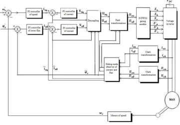
[image:5.612.123.484.354.604.2]

3.1 Sensorless vector control with a sliding mode observer

Figure 1: Block diagram of a vector control with a sliding mode observer

According to the layout diagram of the vector control without mechanical sensor provided with a non-linear observer adaptive by a sliding mode comprising two estimation and adaptation mechanisms one is intended to estimate the speed and the flux, the other is intended for the

(6)

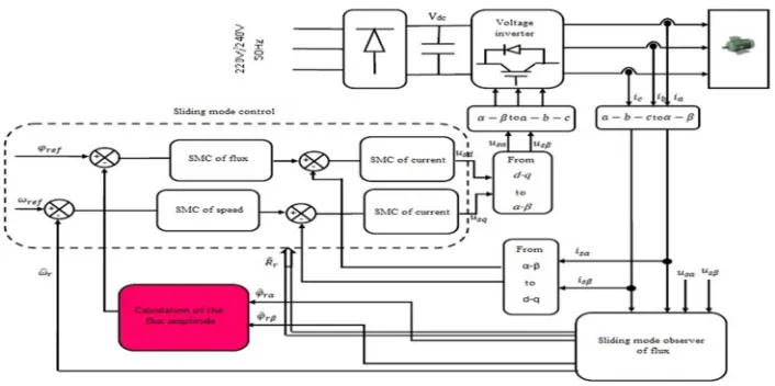
[image:6.612.143.496.149.325.2]

327 3.2 Sensorless Sliding mode control with a sliding mode observer:

Figure 2: Block diagram of a Sliding Mode control with a sliding mode observer

In order to highlight the performances of the sliding mode observer applied to the sliding mode control without mechanical sensors. The scheme of the implementation of the sliding mode control with a sliding mode observer is identical to the last except that the four PI controllers we change them by four sliding mode controllers.

4. DESING OF SLIDING MODE

OBSERVER USING XILINX SYSTEM GENERATOR

XSG is a tool box developed by Xilinx to be integrated into the MATLAB-Simulink environment and allows users to create highly parallel systems for FPGAs. The models created are displayed as blocks and can be linked to other blocks and all other boxes MATLAB-Simulink tools. Once the system is completed, the VHDL code generated by the XSG tool replicates exactly the behavior observed in MATLAB. It is much easier to analyze the results with MATLAB than the other tools like ModelSim associated to VHDL. Then, the model may be coupled to virtual engines. The XSG tool is used to produce a model that will immediately work on equipment when completed and validated. In this part we will remake the control algorithms performed using MATLAB-Simulink using the XSG tool. We will complete this paper by a comparative study of the results found with SIMULINK and XSG.

- Design of gains related to the observation of the current:

The matrix of gains related to the observation of the current is given by the following expression:

A A A"

A$ A% D δ

0 0 δ"

H J

R

σL L σLω

ω

σL σL L KR

L δ 0

0 δ"

Because the XSG environment does not accept analytical expressions we then calculate the terms of the matrix:

A _{σL L δ}R _{0.0929 ∗ 0.462 ∗ 0.462 . 80}4.2

16944.923 A" 0

A$ 0

A% _@A>₎?_A_?δ" _{‚.‚ƒ"ƒ∗‚.%„"∗‚.%„"}%." . 80

16944.923

- Design of gains related to the observation of the flux:

The matrix of gains related to the observation of the flux is given by the following expression:

A& A_A& _&$ A_A&"_&% q₀δ _q0 "δ"

(7)

328

A&" A&$ 0

A&% q"δ" 10 ∗ 80 800

The design of the sub block concerning to the determination of the gains related to the

[image:7.612.89.291.451.576.2]

observation of the flux, and the observation of the current with the XSG environment of Xilinx is given by the figure below:

Figure 3: Schema of the sub block: calculating of the gains related to the observation of the flux and the observation of the currents

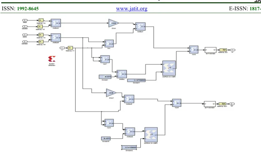
- Design of Sub block of calculation

of current:

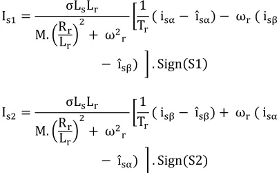
According to the theoretical study developed previously (8) we can write:

I σL L

M. 'RL ," ω" x

1

T i ı̂ ω i

ı̂ y . Sign S1

I" σL L

M. 'RL ," ω" x

1

T i ı̂ ω i

ı̂ y . Sign S2

By substituting the numerical values we obtain:

I _{36.35 ω}0.0198_" _{q9.09 i} ı̂ ω i

ı̂ s Sign S1

I" _{36.35 ω}0.0198" _{q9.09 i} ı̂ ω i

ı̂ s Sign S2

(8)

[image:8.612.88.505.68.310.2]

329

Figure 4: Scheme of subblock: calculation of stator currents designed by XSG

So we designed all sub blocks of the sliding mode observer of the flux and the stator currents. We will collect them, connect them and realize the overall scheme of our observer realized in the XSG environment is shown in figure 5.

Figure 5: Overall scheme of the block of the sliding mode observer designed with the tool XSG

5. SIMULATION RESULTS

5.1. Sensorless vector control with a sliding mode observer

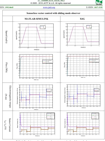
To test the performance and robustness of the sensorless vector control with a sliding mode observer in different areas of functioning, we will perform a series of tests on the variation of different grandeur of machine: (speed, load).

• 1st test: speed variation and application of a load torque

[image:8.612.115.527.385.568.2]

(9)

330

Sensorless vector control with sliding mode observer

MATLAB-SIMULINK XSG

S p ee d ( ra d /s ) F lu x ( W b ) E le ct ro m ag n et ic to rq u e (N .m ) S ta to r C u rr en t i sd , i

sq₍

A

[image:9.612.94.532.51.642.2]

)

Table 1: Simulation results of the sensorless vector control with a sliding mode observer

For this first test we note well:

- For the curve of speed, it is clear that the speed follows the setpoint even by reversing the direction of rotation.

- For the flux curve, we see that the actual flux and the flux observed follow well the reference flux.

- For the electromagnetic torque curve, it is clear that it is the image of the stator current along the axis q. From where the decoupling is assured

0 0.5 1 1.5 2

-20 0 20 40 60 80 100 120 time(s) sp ee d ( ra d /s ) W W_ref

0 0.5 1 1.5 2

-20 0 20 40 60 80 100 120 time(s) sp ee d ( ra d /s ) W Wref

0 0.2 0.4 0.6 0.8 1 1.2 1.4 1.6 1.8 2

0 0.1 0.2 0.3 0.4 0.5 0.6 0.7 0.8 0.9 1 time (s) F lu x ( W b ) Flux observed Flux real Flux of reference

0 0.2 0.4 0.6 0.8 1 1.2 1.4 1.6 1.8 2

0 0.1 0.2 0.3 0.4 0.5 0.6 0.7 0.8 0.9 1 time (s) F lu x ( W b ) Flux observed Flux real Flux of reference

0 0.2 0.4 0.6 0.8 1 1.2 1.4 1.6 1.8 2

-6 -4 -2 0 2 4 6 8 10 12 time(s) E le c tr o m ag n e ti c to rq u e (N .m ) C em Cr

0 0.2 0.4 0.6 0.8 1 1.2 1.4 1.6 1.8 2

-6 -4 -2 0 2 4 6 8 10 12 time(s) E le ct ro m ag n et ic t o rq u e (N .m ) Cem Cr

0 0.2 0.4 0.6 0.8 1 1.2 1.4 1.6 1.8 2

-1 0 1 2 3 4 5 6 7 8 time(s) S ta to r C u rr en t (A ) isdobserved isqobserved isdreal isqreal

0 0.2 0.4 0.6 0.8 1 1.2 1.4 1.6 1.8 2

(10)

331 between the torque and flux. And applying of a load torque at t = 0.6s affects well the value of the current

- For the curve of the observed stator current, we note well that the observed values and real curves are identical

- For curves designed by XSG we see that they are identical to those given by SIMULINK.

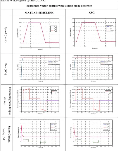
• 2nd test: low-speed functioning:

To test the observability of our system at very low speeds we operate the machine at a low speed and we apply a reverse ramp of speed at t = 1s to reach a value of 3 rad / s at t = 1.3 s and we apply a zero as a load torque Cr = 0.

Sensorless vector control with sliding mode observer

S p ee d ( ra d /s ) F lu x ( W b ) E le ct ro m ag n et ic to rq u e (N .m ) S ta to r C u rr en t i sd , i

sq₍

A

[image:10.612.109.516.191.706.2]

)

Table 2: Simulation results of the sensorless vector control with a sliding mode observer

0 0.5 1 1.5 2

-20 0 20 40 60 80 100 120 time(s) S p ee d ( ra d /s ) W obs W ref W real

0 0.5 1 1.5 2

-20 0 20 40 60 80 100 120 time(s) S p ee d ( ra d /s ) Wobs Wref W real

0 0.2 0.4 0.6 0.8 1 1.2 1.4 1.6 1.8 2

0 0.1 0.2 0.3 0.4 0.5 0.6 0.7 0.8 0.9 1 time(s) F lu x ( W b ) Flux observed Flux real Flux of reference

0 0.2 0.4 0.6 0.8 1 1.2 1.4 1.6 1.8 2

-0.8 -0.6 -0.4 -0.2 0 0.2 0.4 0.6 0.8 1 time(s) E le ct ro m ag n et ic t o rq u e ( N .m ) _C em Cr

0 0.2 0.4 0.6 0.8 1 1.2 1.4 1.6 1.8 2

-0.8 -0.6 -0.4 -0.2 0 0.2 0.4 0.6 0.8 1 time(s) E le ct ro m ag n et ic t o rq u e ( N .m ) _C em Cr

0 0.2 0.4 0.6 0.8 1 1.2 1.4 1.6 1.8 2

-2 0 2 4 6 8 10 time(s) S ta to r C u rr en t( A ) isdobs isqobs isdreal isqreal

0 0.2 0.4 0.6 0.8 1 1.2 1.4 1.6 1.8 2

(11)

332 For this second test at low speed we note although:

- The speed curve follows well its reference value even at low speeds. By performing the zoom the difference is negligible.

- the curves of flux observed and the actual flux follow very well the curve of flux of reference.

- We note that the electromagnetic torque is the image of the stator current along the axis q. So we checked well decoupling between torque and flux.

5.2. Sensorless sliding mode control with a sliding mode observer

For the speed setpoint, we start with the magnetization regime of the machine, then we apply a ramp of speed at t = 0.1s to reach its reference value (100 rad / s) at t = 0.3s. Then, at t = 1.2s we apply a negative speed to the machine reaching a value of (-50 rad / s) at t = 1.2s. The nominal value of the reference flux is equal to 0.9 Wb.

Sensorless sliding mode control with sliding mode observer

S p ee d ( ra d /s ) F lu x ( W b ) E le ct ro m ag n et ic to rq u e (N .m )

0 0.5 1 1.5 2

-20 0 20 40 60 80 100 120 time(s) sp e ed ( ra d /s ) W W ref

0 0.5 1 1.5 2

-20 0 20 40 60 80 100 120 time(s) sp ee d ( ra d /s ) W Wref

0 0.2 0.4 0.6 0.8 1 1.2 1.4 1.6 1.8 2

-0.8 -0.6 -0.4 -0.2 0 0.2 0.4 0.6 0.8 1 time (s) E le ct ro m ag n et ic t o rq u e (N .m ) C em C r

0 0.2 0.4 0.6 0.8 1 1.2 1.4 1.6 1.8 2

(12)

333

Table.3: Simulation results of the sensorless sliding mode control with a sliding mode observer

According to these results obtained by performing these tests, we can conclude that the sliding mode control with the sliding mode observer gives very satisfactory results. This sensorless control demonstrated a good robustess against parametric variations. This type of control has displayed a perfect decoupling between flux and torque. And the most important that the results obtained with the XSG environment are similar to those obtained with SIMULINK. So this type of control can immediately be implemented on FPGA

6. CONCLUSION

In the first part of this paper, we presented the approach of the sliding mode observer. Then we focused on the importance of sensorless control in order to increase the profitability of our machine.

After we applied this observer to the vector control and the sliding mode control.

At the end, a comparison was made between the results obtained with XSG and Simulink and we can conclude that the results obtained by these two environments are the same therefore our algorithms can be implemented on the FPGA board. In addition, by performing several tests: speed control, speed reversal, applying a load torque we can conclude that the sliding mode observer meets the most critical needs of the control laws of the MAS of the viewpoint of robustness against parametric variations and ensures proper operation over all the entire speed range especially during low speed operation. mode control. In the third part of this paper, we designed the sensorless controls with XSG to implement them on the FPGA board.

Finally, this tool XSG allowed us to solve many problems in the field of machine control. All his problems are related to difficulties in using VHDL. With this graphical environment all his problems are solved. but as a perspective of this work we must think seriously about developing a

comprehensive library under XSG similar to Simulink based on the principle of reusability and future work thinking to develop methods to further optimize the algorithms designed with 'XSG tool in reducing the number of resources used and the computation time. Because the major drawback of this method: it gives non-optimized algorithms when use the material resources of the FPGA

REFRENCES:

[1] Jemli M., Ben azza H., Boussak M., Gossa M., "Sensorless indirect stator field orientation speed control for single-phase induction motor drive, IEEE Transaction Power Electronics, Vol.24, Issue 6, pp.1618-1627, 2009.

[2] Trabelsi R., Khedher A., Mimouni M.F., M'sahli F., 'Backstepping control for an induction motor using an adaptive sliding rotor-flux observer', Electric Power System

Research, Elsevier, 2012.

[3] Dunningan M.W., Wade S., Williams B.W. Yu X., 'Position control of vector controlled induction machine using Slotine's sliding mode control approach', IEEE Proccedings on Electrical Power Applications, on Industrial

Electronics, Vol.145, Issue 3, pp. 231-238,

1998.

[4] Trabelsi R., Khedher A., Mimouni M.F., M'sahli F., Masmoudi A., 'Rotor flux estimation based on non linear feedback intergrator for backstepping controlled induction motor drives.' Electromotion, Vol.17, Issue 3, pp. 163-172, 2010.

[5] Negadi K., Mansouri A., Khtemi B., "Real time implementation of adaptive sliding mode observer based speed sensorless vector control of induction motor" , Serbian Journal of Electrical Engineering, Vol.7, N°2, November 2010, pp. 167-184.

S

ta

to

r C

u

rr

en

t

i

sd

, i

sq₍

A

)

0 0.2 0.4 0.6 0.8 1 1.2 1.4 1.6 1.8 2

-1 0 1 2 3 4 5 6 7 8

time(s)

S

ta

to

r

C

u

rr

en

t(

A

)

isqobs isdobs isqreal isdreal

0 0.2 0.4 0.6 0.8 1 1.2 1.4 1.6 1.8 2

-1 0 1 2 3 4 5 6 7 8

time(s)

S

ta

to

r

C

u

rr

en

t(

A

)

(13)

334 [6] Traoré D., De Leon J., Glumineau A. , Loron

L., "Interconnected observers for sensorless induction motor in dq frame : Experimental tests", IECON, Paris, France, pp. 5093-5100, November 7 - 10, 2006.

[7] Ghanes M., Girin A., Saheb T., "Original Benchmark for sensorless induction motor drives at low frequencies and validation of high gain observer", IEEE American Control Conference ACC'04, Boston, Massachussets, USA, 30 juin-2 juillet 2004.

[8] Soltani J., Payan A.F., Abassian M.A., "A speed sensorless sliding mode controller for doubly fed induction machine drives with adaptive backstepping observer, IEEE

International Conference on Industrial

Technology, ICIT 2006, pp. 2725-2730.

[9] Utkin V.I., "Sliding modes in control and optimization", volume 2. Springer-Verlag, Berlin, 1992

[10]Bossoufi B., Karim M., Ionita S., Largaoui A., "FPGA-Based Implementation with Simulation of Structure PI Regulators Control of a PMSM". International Workshop on Information Technologies and Communication

(WOTTIC’2011), 13-15 October 2011,

Casablanca, Morocco.

[11]Bossoufi B., Karim M., Ionita S., Largaoui A., "Indirect Sliding Mode Control of a Permanent Magnet Synchronous Machine: FPGA-Based Implementation with Matlab & Simulink Simulation" Journal of Theoretical and Applied Information Technology (JATIT), pp. 32-42, Vol.29 N°.1, 15th July 2011.

[12]Gdaim S., Mtibaa A., Mimouni M.F.," Experimental implementation of Direct Torque Control of induction machine on FPGA".

International Review of Electrical Engineering, Vol.8, N°1, ISSN 1827-666, Février 2013.

[13]Charaabi L., Monmasson E., and Belkhodja I., "Presentation of an efficient design methodology for FPGA implementation of control system application to the design of an antiwindup PI controller", In Proceedings IEEE IECON, 2002, pp. 1942–1947.

[14]Chapuis Y.A., Blonde J. P., Braun F., "FPGA Implementation by Modular Design Reuse mode to Optimize Hardware Architecture and performance of AC Motor Controller Algorithm". In Proceedings, EPE-PEMC Conference., September. 2004.

[15]Rajendran R., Devarjan N., "FPGA based implementation of space vector modulated Direct Torque Control for induction motor drive". International Journal of Computer and Electrical Engineering, Vol.2, N°3, ISSN 1793-8163, June 2010.

[16]Rajendran R., Devarjan N., "Simulation and implementation of a high performance torque control scheme of IM utilizing FPGA".,

International Journal of Computer and Electrical Engineering (IJECE), Vol.2, N°3,

ISSN 2088-8708, pp. 277-284, June 2012.

[17]Monmasson E., Cristea M., "FPGA Design Methodology for Industrial control systems- A

Review IEEE trans. Ind. Electron.., Vol.54 N°4, pp.1824-1842, August 2007.

[18]Lis J., Kowalaski C.T., Orlowaska-Kowalaska T., " Sensorless DTC control of the Induction motors using FPGA", International Symposium on Industrial Electronics, June 30 2008- July 2 2008. IEEE 2008.