Munich Personal RePEc Archive
Disposition effect and gender
Newton, Da Costa Jr and Carlos, Mineto and Sergio, Da
Silva
Federal University of Santa Catarina
2006
Online at
https://mpra.ub.uni-muenchen.de/1848/
Disposition effect and gender
Newton Da Costa, Jr
Department ofEconomics, Federal University of Santa Catarina Florianopolis SC 88049-970, Brazil
and Pompeu Fabra University, Spain
Carlos Mineto
Staff, Pontifical Catholic University of Parana Curitiba PR 80215-901, Brazil
Sergio Da Silva
Department of Economics, Federal University of Santa Catarina Florianopolis SC 88049-970, Brazil
[email protected] Corresponding author
Abstract
Investors seem to hold on to their losing stocks to a greater extent than they hold on to their winning stocks. This well-document behavioral regularity is termed disposition effect (Shefrin and Statman 1985). We set an experiment to replicate results from a previous study of the disposition effect (Weber and Camerer 1998), and further show that a subject’s gender may interfere with the effect’s detection.
JEL Classification: G11
1. Introduction
Investors seem to hold on to their losing stocks to a greater extent than they hold on to their winning stocks. This well-document behavioral regularity is termed disposition effect (Shefrin and Statman, 1985). The effect is usually explained by utility assumptions of loss aversion (Kahneman and Tversky, 1979). When judging gains and losses relative to a starting reference point (such as purchasing price), investors are risk averse toward gains and risk seeking toward losses (Weber and Camerer, 1998).
A changing reference point also alters the disposition effect. Yet once one allows the reference point to shift there is no extra need for assuming loss aversion (Grinblatt and Han, 2002). A complete rationale for the disposition effect taking changing reference points into account demands extending Kahneman and Tversky’s prospect theory to consider risky choices in an intertemporal framework. Here Loewenstein and Prelec (1992) generalize discounted utility theory and set an intertemporal prospect theory. They also sketch an explanation for the disposition effect, though they do not consider changing reference points. It is as follows. The value function is convex in the loss domain, and then losses are less than proportionately painful. And gains yield marginally increasing returns. Thus there are incentives to holding on to the stock. The incentives are reversed on the gain side, motivating investors to quickly sell stocks that have gained in value (Loewenstein and Prelec, 1992, p. 594). (Comprehensive references on the disposition effect are provided elsewhere (Weber and Camerer, 1998)).
An alternative to intertemporal loss aversion in explaining the disposition effect is plain mean-reversion. Investors might keep losing stocks just because they rationally guess they will gain in value in future.
Ultimate tests proving the disposition effect in actual markets are difficult because investors’ decisions and expectations cannot be controlled in there. Experiments can be run instead. An experiment can be designed to match individual investors’ trading decisions with the prices at which they buy the stocks. Here we replicate such an experiment (Weber and Camerer, 1998) only to find that a subject’s gender interferes with the disposition effect’s detection.
Generally gender differences may be involved in risk-taking (Byrnes et al., 1999). If anything, women are more risk-averse. Yet experimental studies suggest women’s risk aversion to be framing dependent (Schubert et al.,2000). In line with the latter we find the disposition effect in female subjects to vary with changing reference points.
Section 2 presents the hypotheses to be tested. Section 3 describes the experiment design. Section 4 presents results. And Section 5 concludes.
2. Hypotheses
The hypotheses in Weber and Camerer’s (1998) experiment are as follows.
H1 Subjects sell more (less) stocks when the sale price is above (below) the purchasing price.
H2 Subjects sell more (less) stocks when the sale price is above (below) the previous price.
Selling a stock requires a deliberate action. Yet one can imagine an automatic selling at the end of a period. Here subjects will repurchase the stocks at the same price they were automatically sold for. Since rational investors will make no distinction between deliberate and automatic selling it is implied that
H3 Subjects selling stocks deliberately show greater disposition effect than subjects selling stocks automatically.
Here we will find hypotheses H1 and H3 to hold. Yet H2 will collapse for female subjects.
3. Experiment design
Subjects were asked to make portfolio decisions prior to each of 14 periods. They had to buy or sell six stocks (A, B, C, D, E, and F) at pre-announced prices. Each subject was endowed with fictitious 60,000 Brazilian reais (~ US$25,000). A stock had to be bought at R$10,000 each. Subjects could neither borrow nor sell short, and were not allowed to diversify their portfolios. (No real money were involved, unlike in Weber and Camerer's where a tiny fraction of gains was paid; but even with no monetary reward we were able to reproduce their results.)
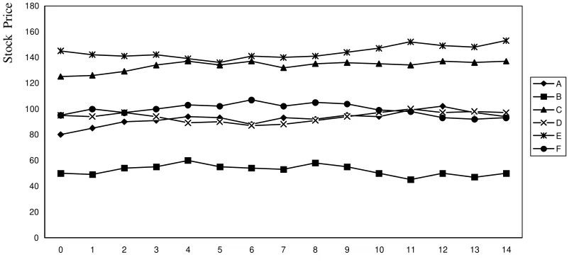
Prices were generated randomly rather than being the result of subjects’ actions. This aims at isolating a possible disposition effect (where there is a tendency to buy and sell at distinct prices) from the process of price formation. Prices were then announced on two stages. (1) Each period a price could rise or fall according to the probabilities in Table 1. Subjects were informed of these chances of price rising or falling, but they still had to guess which stock (A−F) had which probability of price increase. They reported their guesses on a questionnaire distributed in white sheet for male and pale-pink sheet for female subjects. (2) Being known whether an increase or drop were involved, the size of price rise or fall (whether R$1, R$3, or R$5) was determined randomly. Figure 1 shows the resulting price series.
4. Results
To examine H1 we consider a first-in-first-out (FIFO) setting, where the stocks sold are those bought at the beginning. To consider H2 we take a last-in-first-out (LIFO) setting, where the stocks sold are those bought at the end of previous period.
Table 2 shows results for the FIFO setting. Overall the disposition effect is present. Here our null hypothesis is the number of sales with gain to be less or equal to the number of sales with loss. We found 63 percent of all trades to result in gains and only 34 percent to end up in losses. Trading stocks D and E were exceptions, exactly as in Weber and Camerer's. (A Z statistics of 13.30 was significant at less thanone percent.)
Table 3 shows more stocks to be sold as the previous prices increase. More than half of all trades (60 percent) occur taking the last price as reference (Z = 8.28, p < 0.01). Thus the disposition effect is heightened when the purchasing price is compared to previous prices. Yet table 4 shows the disposition effect to vanish when automatic selling is allowed. Relatively more trades yield losses (50.1 percent). This confirms H3 and is also in line with Weber and Camerer’s findings.
H3 can also be evaluated for individual subjects by means of a disposition coefficient α =
(
S+−S−) (
S++S−)
, where S+(S−) is the number of sales following a higher (lower) price at the previous period. The coefficient is zero if the number of stocks sold on with gain matches the number sold on with loss, in which case there is no disposition effect. The coefficient is +1 (−1) if a subject sells on following a gain (loss). For experiment I, we found αI = 0.095 (t = 1.80, p = 0.075, one-tailed t-test). And forexperiment II, the disposition coefficient was not significantly different from zero (αII = –
0.0023).
Considering gender differences does not matter for sale decisions using the purchasing price as a reference point. Here the disposition effect in male and female subjects shows no significant difference (Tables 5a and 5b).
Yet gender interferes with H2. When reference point is the previous price the disposition effect still occurs with males but vanishes for female subjects (Tables 6a and 6b). For male subjects α = 0.351 (t = 4.41, p < 0.01, one-tailed t-test). And for the average of 52 female subjects the coefficient is negative, but nonsignificant for a one-tailed t-test(α = −0.172).
We speculate that female decisions violating H2 are brain-wired. According to empathizing-systemizing theory (Baron-Cohen, 2002), due to superior visuospatial memory (i.e. the ability to remember the relative locations of objects) women do a first-class job of remembering landmarks. This contrasts with reading maps, which is a specialty of the male “systemizing” brain. Thus male and female brains might interpret changing reference points differently. Yet the issue is only likely to be settled using brain-scanning experiments, such as fMRI.
positively autocorrelated. Yet boys show behavior consistent with mean-reversion (negative autocorrelation).
5. Conclusion
Figure 1. Stock prices pre-announced in the experiment
Table 1. Probabilities of Stock Price Increase
Stock A B C D E F
Probability of Price Increase (%) 35 45 50 50 55 65
Symbol − − − 0 0 + + +
Table 2. Testing H1. Sales with the Purchasing Price as the Reference Point
Stock A B C D E F Overall*
Total % Total % Total % Total % Total % Total % Total % Sales with Gain 314
81 210 54 253 87 167 46 127 44 219 68 1290 63
Even 50
13
50
2
Sales with Loss 72
19 128 33 39 13 197 54 159 56 101 32 696 34
Total 386 388 292 364 286 320 2036 Note
* Z = 13.30, p-value < 0.01 for the test of gains (1290) versus losses (696)
0 20 40 60 80 100 120 140 160 180
0 1 2 3 4 5 6 7 8 9 10 11 12 13 14
Table 3. Testing H2. Sales at t Using Previous Prices at t− 2 and t− 1 as Reference Points Experiment I: Deliberate Sales
Price Stock Trend
A B C D E F Overall* %
t− 2 t− 1
G G 84 65 57 61 65 30 362 L G 20 42 16 78 − G 107 101 102 103 82 74 569 Total 191 166 179 206 147 120 1009 60
G L 25 24 6 11 28 94 L L 47 37 17 26 39 34 200
− L 72 77 39 65 50 72 375
Total 144 138 62 91 100 134 669 40
Note
G = gain, L = loss
* Z = 8.28, p-value < 0.01
Table 4. Testing H3. Sales at t Using Previous Prices at t − 2 and t − 1 as Reference Points
Experiment II: Automatic Sales
Price Stock Trend
A B C D E F Overall* %
T− 2 t− 1
G G 206 138 153 135 130 56 818 L G 0 0 21 88 0 21 130 − G 234 173 207 223 179 105 1121
Total 440 311 381 446 309 182 2069 49.9
0 0 0 0 0 0 0 G L 104 78 32 0 41 88 343
L L 66 143 68 62 111 145 595 − L 170 257 162 129 152 273 1143
Total 340 478 262 191 304 506 2081 50.1
Note
[image:8.612.87.446.362.584.2]Table 5a. Female Sales Using the Purchasing Price as a Reference Point
Stock A B C D E F Overall*
Total % Total % Total % Total % Total % Total % Total % Sales with Gain 141
71 76 44 97 78 78 39 51 38 82 61 525 55
Even 23
13
23 2 Sales with Loss 57
29 73 42 27 22 120 61 83 62 53 39 413 43
Total 198 172 124 198 134 135 961 Note
* Z = 3.69, p-value < 0.01 for the test of gains (525) versus losses (413) Table 5b. Male Sales Using the Purchasing Price as the Reference Point
Stock A B C D E F Overall*
Total % Total % Total % Total % Total % Total % Total % Sales with Gain 173
92 134 62 156 93 89 54 76 50 137 75 765 71
Even 27
13
27
3
Sales with Loss 15
8 55 25 12 7 77 46 76 50 45 25 280 26
Total 188 216 168 166 152 182 1072 Note
* Z = 14.97, p-value < 0.01 for the test of gains (765) versus losses (283)
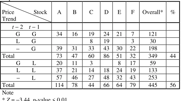
Table 6a. Female Sales at t Using Previous Prices at t− 2 and t− 1 as Reference Points Experiment I: Deliberate Sales
Price Stock Trend
A B C D E F Overall* %
t − 2 t − 1
G G 34 16 19 24 21 7 121
L G 8 19 3 30
− G 39 31 33 43 30 22 198
Total 73 47 60 86 51 32 349 44
G L 20 11 3 8 17 59 L L 37 21 14 18 24 19 133 − L 57 46 27 48 32 43 253
Total 114 78 44 66 64 79 445 56
Note
* Z = −3.44, p-value < 0.01
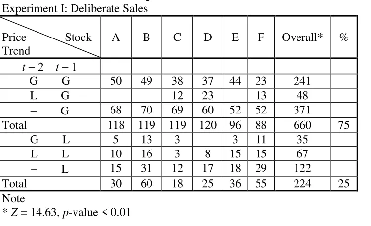
Table 6b. Male Sales at t Using Previous Prices at t− 2 and t− 1 as Reference Points Experiment I: Deliberate Sales
Price Stock Trend
A B C D E F Overall* %
t− 2 t− 1
G G 50 49 38 37 44 23 241
L G 12 23 13 48
− G 68 70 69 60 52 52 371 Total 118 119 119 120 96 88 660 75
G L 5 13 3 3 11 35 L L 10 16 3 8 15 15 67 − L 15 31 12 17 18 29 122
Total 30 60 18 25 36 55 224 25
Note
* Z = 14.63, p-value < 0.01
Table 7. Gender and Mean-Reversion
Subject’s Gender Prices Rising at t− 1 (%) G
Prices Falling at t− 1 (%) L
Overall 47 53*
Male 34 66**
Purchases at t
Female 61 39
Notes
To check for mean-reversion, we test whether subjects buy more losing stocks (L) than winners (G)
[image:10.612.78.536.350.434.2]References
Baron-Cohen, S. (2002) The extreme male brain theory of autism, Trends in Cognitive Sciences, 6, 248-54.
Byrnes, J. P., D. C. Miller, and W. D. Schafer (1999) Gender differences in risk-taking: a meta-analysis, Psychological Bulletin,125, 367−83.
Grinblatt, M., and B. Han (2002) The disposition effect and momentum, NBER Working Paper, 8734.
Kahneman, D., and A. Tversky (1979) Prospect theory: an analysis of decision under risk,
Econometrica, 47, 263−91.
Loewenstein, G., and D. Prelec (1992) Anomalies in intertemporal choice: evidence and an interpretation, Quarterly Journal of Economics, 107, 573−97.
Schubert, R., M. Gysler, M. Brown, and H. W. Brachinger (2000) Gender specific attitudes towards risk and ambiguity: an experimental investigation, Swiss Federal Institute of Technology Working Paper.
Shefrin, H. M., and M. Statman (1985) The disposition to sell winners too early and ride losers too long, Journal of Finance, 40, 777−90.