Reduction of Continuous Neuronal Model to Discrete Binary Automata

Reduction of Continuous Neuronal Model

to Discrete Binary Automata

Abir Hadriche

Laboratory of Electronics and Information Technologies Sfax university, Sfax, Tunisia.

and

Institut de Neurosciences des Syst `emes (UMR S 1106) Aix-Marseille University, INSERM, Marseille, France.

Nawel Jmail, Hamadi Ghariani, Abdennaceur Kachouri

Sfax University, Sfax, Tunisia.

Laurent Pezard

Institut de Neurosciences des Syst `emes (UMR S 1106) Aix-Marseille University, INSERM, Marseille, France.

ABSTRACT

This article presents the reduction of neuronal models from the classic four-dimensional differential model of Hodgkin and Huxley [7] to discrete binary automata which keep the main properties of more complex models. A reduction of Fitzhugh and Nagumo (FHN) model is performed using a numerical strategy introduced in [3] completed by a linearization in the spirit of McKean model [14]. The resultant discrete binary model keeps the properties of the complete FHN model. The numerical simulations of networks composed by these discrete binary automata demonstrate changes in the system dynamics dependent on the coupling strength. Moreover, for large coupling strength, phase-locking is observed.

General Terms:

neuronal modeling, discrete model

Keywords:

neuronal models, Hodgkin and Huxley model, FitzHugh Nagumo model, binary model, time discrete reduction

1. INTRODUCTION

Brain functioning depends on several scales of organization from molecules to the entire brain which also act at several temporal scales. As a consequence, the nervous system is one of the typical complex system. Although neuroscience offers a large set of recording techniques of brain activity, major advances in the comprehension of brain functioning may depend on the ability to simulate brain activity and to obtain theoretical results for further investigation.

The study of neuronal excitability by Hodgkin and Huxley [7] has provided one of the major advance towards the integration of physiological and theoretical perspectives for the understanding of neural network functions. Nevertheless the use of Hodgkin and Huxley (HH) model to simulate brain functioning is

noticeably difficult due to high demand in computation (see [10]). There is thus a crucial need to obtain simpler models of neuronal activity in order to deal with models reasonable all together in computational demand, analytic tractability and biological realism. This is usually achieved by hybrid spiking models [9] which comprise the integrate-and-fire models family. The reduction of the continuous models of neural dynamics to dynamics discrete in both state and time complements the hybrid models but is less widely used. Nevertheless, these discrete models keep important properties of neuronal dynamics [1, 15, 11] and may offer a general framework for the study of large-scale neuronal networks. Moreover, the development of discrete automata analogs of neuronal dynamics may prove the same interest as the one depicted by cellular automata as models of physical systems [4].

In the first part of this paper, the reduction of HH model to two dimensional continuous models is rapidly reviewed. This first step allows to introduce the Fitzhugh and Nagumo (FHN) model as a general expression for two-dimensional continuous neuronal models. In the following section, the same strategy as that developed in [3, 2] was used in order to build a binary neuronal analog based on the FHN model. A general method is applied here for the definition of a discrete binary automata model with discrete time dynamics derived from continuous two dimensional continuous model. Simulating this binary model, the behavior is first explored as an isolated automata and compared its properties with those of the continuous FHN model. In a second step, networks of binary automata were simulated. The dynamics of the network in the case of large coupling strength was compared with those obtained in the case of small coupling strength.

2. REDUCTION OF HODGKIN AND HUXLEY MODEL TO TWO-DIMENSIONAL MODEL

the Nobel price, with Sir J. C. Eccles, in 1963 for this important work.

2.1 Hodgkin-Huxley model

The mathematical formulation of the model is based on:

(1) the approximation of the neuron to a point and thus neglecting the spatial dependency of the voltage1

(2) the linear approximation of ionic currents2 _{which thus} follow Ohm’s law, and

(3) the fact that three currents were implied in the explanation of the experimental results: two active ionic currents (sodium and potassium) and one passive leak current.

The conservation of electric charges in squid axon is thus written as:

Cdv

dt =−F+I (1)

wherevis the membrane potential,C is the axon membrane capacitance , I is the sum of external currents entering the cell and F is the total membrane current which arises from the conduction of sodium and potassium ions through voltage-dependent channels in the membrane and the leak current. Each membrane current Ik follows Ohm’s law and is thus

expressed as:

Ik=gk(v−Ek) (2)

whereEk is the reversed potential for the current and gk the

conductance which is constant for the leak current and depends on the kinetics of the ionic channels for the active currents.Fis thus a function of the membrane voltagevgiven by:

F(v, m, h, n) =gL(v−EL)+¯gKn4(v−EK)+¯gN ahm3(v−EN a)

(3) where the subscriptsK,N aandLdenote the potassium, sodium and leakage currents respectively. The variablesn,mandhare voltage-dependent activation and inactivation gating variables assumed to follow first order kinetics. Their dynamics thus take the form:

τw(v) dw

dt =w(v)−w (4)

where w = n, m or h and τw(v) and w(v) are

voltage-dependent time constant and asymptotic value (respectively) determined from the experimental data.

Equations (3) and (4) represent a four dimensional dynamical system which formulates the HH model for action potential genesis. The reduction of this model proceed in two steps which we sum up below.

2.2 Stationary state approximation

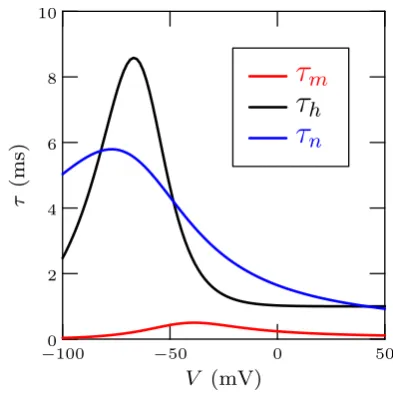
The first step in the reduction of HH model is due to the difference between the time scale of the dynamics of the gating variable m and the time scale of the dynamics of the other variables (see Figure 1). In fact, the time constantτmis lower

than the time constantsτhandτnleading to faster changes for m than forh and n. It can thus be assumed that the gating variablemreaches instantaneously its asymptotic valuem¯(v) and use its value in the expression ofdv/dt. This is equivalent to assuming that activation of theNa+ conductances acts on a time scale even faster than that of the voltage and introduces approximations only for the short time scale of the beginning

1_{This approximation was justified by the experimental technique of the}

voltage clamp which ensures a constant potential on the axon membrane.

2_{This model thus does not take into account the non-linearity which are}

for example present in the Goldman-Hodgkin-Katz equation.

0 2 4 6 8 10

τ

(ms

)

−100 −50 0 50

V

(mV)

τ

_m

τ

_h

τ

n

Fig. 1. Time constant of the dynamics of the gating variables show admissible short time scaleτm.

of the action potential. A new model with three dimensions is obtained:

F(v, m, h, n)≈F(v, m(v), h, n)≡F (5)

This three-dimensional model can be further reduced to a two-dimensional model.

2.3 Reduction to a two-dimensional system

The next step in the reduction of HH model and more generally conductance-based models consists in the study of the relationship between gating variables. In the case of HH model, it can be done at a specific or a general level.

A specific method is based on early numerical simulations of HH model [13] where it was noticed that the sumn(t) +h(t) remains approximately equal to0.84during the time evolution of the system. The variablehcan thus be eliminated by setting

h(t) ≈0.8−n(t)and this led to a two variable model, called the fast-slow phase plane model. Equation (3) can be written as:

F(v, m, h, n)≈F(v, m(v),0.8−n(v), n(v))≡f(v, n) (6)

A general method has been proposed by [3]. It is based on the introduction of an auxiliary variable which represents an equivalent potential. This auxiliary voltage variableuallows to replacehandnby their asymptotic values not at the potentialv

but rather atu. This new variable has a slower time-scale thanv. So equation (5) can be written as:

F(v, m, h, n)≈F(v, m(v), h(u), n(u))≡f(v, u) (7)

This introduction of an equivalent potential has also been used as a general method for the reduction of models based on arbitrary numbers of conductance [12].

2.4 Fitzhugh-Nagumo model

governed by the two differential equations:

εdv

dt =f(v)−u+I (8)

τdu

dt =g(v, u) (9)

whereε depends in capacitanceC, and f(v) and g(u, v)are given by:

f(v) =v−v3/3 and g(v, u) =av+bu (10)

The expression ofdv/dtdefines a fast variable controled by a cubic non-linearity that allows regenerative self-excitation via a positive feedback. The expression of du/dt is linear and provides a slower negative feedback. This model will be used as a basis for the definition of discrete binary automata.

3. FROM FHN NEURONAL MODEL TO DISCRETE BINARY AUTOMATA

The definition of a discrete binary automata based on FHN neuronal model is based on its phase plane analysis3_{and on the} linearization of the cubicv-nullcline.

3.1 Phase plane analysis of FHN model

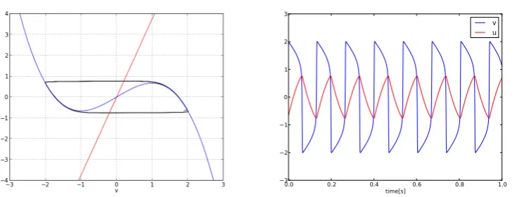
The analysis of FHN model dynamics in the (v, u)-plane is depicted on Figure 2. The behavior of the model is organized around thev−andu−nullclines (i.e.dv/dt = 0anddu/dt= 0). Thev−nullcline has the shape of a cubic function (u=v−

v3_{/3 +I) and theu−nullcline is a linear function (u=−av/b).}

The intersection point of these nullclines define the fixed points of the dynamics.

The stimulus current I acts as a control parameter since it shifts thev−nullcline on the vertical axis and thus changes the dynamics in the neighborhood of the fixed point. In this paper, the case where the two nullclines intersect on the ascending parts of the cubic nullcline (e.g.I = 0) will be applied. In this case, the fixed point is unstable and the system evolves on a limit cycle which leads to repetitive firing4_.

The dynamics of the membrane voltagevduring the firing of action potential is composed offast phaseswhere the voltage change from low values to high values and reciprocally and slow phaseswhere the voltage has high or low values. The slow phases last longer than the fast phases and thus FHN model evolves mainly along the v−nullcline, while changes of the membrane voltage levels are almost instantaneous (see Figure 2). This remark is the starting point of the further analysis which leads to the discrete binary model [3].

3.2 Reduction of FHN model

On the basis of the previous remark, one can consider that the membrane potential can have either a high or a low value and changes instantaneously between these two levels. This approximation corresponds to neglecting the capacitance of the membrane. Moreover, when the membrane potential evolves on either of these levels:dv/dt≈0. On the basis of this hypothesis,

3_{Only the main points of the phase plane analysis of FHN model are}

summed up here; for a more complete analysis see: [6].

4_{The difference between FHN model and that developed in [3] lay in the}

fact that only the left hand portion of thev-nullcline curve rises asIis increased in the case of the latter whereas the entire curve is translated in the case of FHN model. This causes an independence between the firing frequency and the action potential amplitude in the case of FHN model whereas the amplitude of the action potentials decrease when firing rate increase in the other model as in full HH model.

one can thus rewrite equation (8) as:

dv

dt =f(v)−u+I≈0 (11)

When the model is on one of these levels, it evolves on one of the branches of the cubic shapedv−nullcline. In the spirit of McKean model [14] thev−nullcline can be assimilated to a piecewise linear function which allows to simplify its cubic shape: the left and right branch in the cubic are replaced by two straight lines. An approximation of these lines is given by observing that the dynamics remains in the neighborhood of the minimum and the maximum of the cubic nullcline. These extrema form right and left knees of the curve with coordinates:

l= (−1,−2/3 +I)andr= (1,2/3 +I).

The linear approximation should thus intersect a knee and depict a slopeas <0close to the best fit of the portion of the cubic

followed by the system during the slow phases. The two straight segments can thus be expressed as:

nl(v) =asv+bs+I forv≥1 (12)

nr(v) =asv−bs+I forv≤ −1 (13)

wherebs = 2/3−as. In the numerical examples, the values as=−1.5and thusbs= 2.16were used (see figure (3)).

Now a binary variableScan be introduced to keep track of which branch of the curve is being used [3, 2].

S=

(

+1 ifv≥1,

−1 ifv≤ −1. (14)

There is no need to defineS in the region wherevis between −1 and 1 because in the limit of small cell capacitance, the membrane potential jumps instantaneously over this region, always remainingv >1in absolute value [1].

Equations (12) and (13) can then be written as:

n(v) =asv+Sbs+I (15)

and using (15) to solve (11) forv:

v=u−bsS−I

as

(16)

and one can rewrite (9) as:

τdu

dt =a

u−bsS−I as

+bu (17)

SinceS=sign(v−S), the binary variableScan be expressed by:

S=sign

u−(2S/3)−I

as

(18)

and equations (17) and (18) constitute the binary analog of the FHN model. The variableS is the controlled discretization of the state variablev. Thus, if the cell is hyperpolarised and silent:

S=−1and, if it is depolarized and firing:S= +1.

4. NUMERICAL SIMULATIONS

For numerical applications,as =−1.5and thusbs = 2.16are

used, leading to the following system:

τdu

dt =a

I−u+ 2.16S

1.5

+bu (19)

S=sign[0.66S−u+I] (20)

4.1 Single cell behavior

In order to demonstrate the behavior of one neuron, a discrete time version of the model can be generated by integrating equations (18) and (17) over one time step4t:

0.0 0.2 0.4 0.6 0.8 1.0 time[s]

3 2 1 0 1 2 3

v u

Fig. 2. Phase portrait and time series of the FHN model plotted with these Parameters:a= 0.75;b=−0.2;I= 0;τ= 50;= 1.

Fig. 3. The two approximated straight lines of the cubic shape of FHN model. These two lines are the tangents of each branch which

intersected respectively the two knees of the cubic.

The functionu(t)representing the slow component of the cell membrane current has be discretized by solving (17) as a first order differential equation of the unknownu:

u(t+4t) =u(t)exp(−C1

τ 4t) +

C1

C2

1−exp(−C1

τ 4t)

(22) with:C1=−b+a/1.5andC2=a(I+ 2.16S)/1.5.

The results of the numerical simulation of this model are depicted on Figure 4 and can be compared with those obtained for the continuous FHN model with the same parameters depicted on Figure 2.

4.2 Behavior of networks of discrete binary automata

Networks ofN discrete binary automata are simulated using equations (19) and (20) and discrete time with stepsδt= 1ms. Each automata is characterized by a binary variablesSi and a

recovery variableui withi = 1. . . , N. The state of celliis

updated at timet+ 1using:

Si(t+ 1) =sign[Si(t)−ui(t) +Ii(t)] (23)

whereIi(t)is the sum of the synaptic input to neuroniat timet

and defined as in the Hopfield model [8]:

Ii(t) =

1

N N

X

j=1

JijSj(t) (24)

withJij is the element of the N ×N matrix J of synaptic

coupling from neuron j to neuron i. The magnitude of Jij

determines the strength of the coupling betweenjandiand its sign describes whether the synapse is excitatory or inhibitory. Network behavior can be characterized using the alignment of the stateSiat timetby introducing the variable [2]:

m(t) = 1

N N

X

i=1

Si(t) (25)

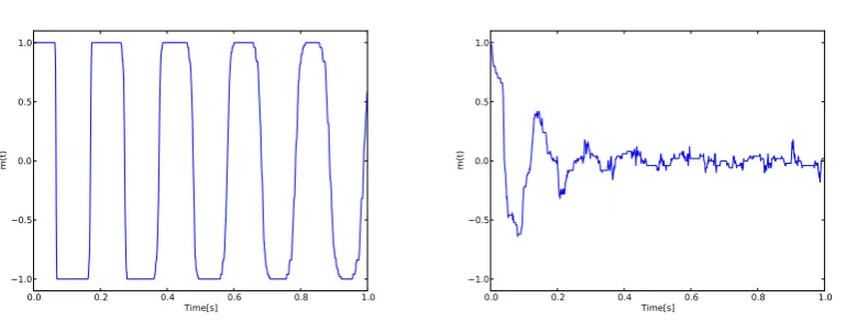
The averageshm(t)iandhm2_{(t)iare equal to zero in the case}

of disordered dynamics whereas in the case of phase-locking: hm(t)i= 0buthm2_{(t)i 6= 0[2].}

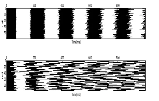
The dynamics of two types of networks of discrete binary automata were studied: one with strong coupling strength (see Figure 5) and one with weak coupling strength (see Figure 6).

For strong coupling,Jijare randomly drawn from an uniform

distribution on the interval[−1,1]. For weak coupling, they are drawn from an unform distribution on the interval[−0.03,0.03]. In the case of strong coupling, one can observe coherent oscillations and the network maintains some particular pattern of activity. In this casehm2_{(t)i= 0.72and signs the presence}

of phase-locking in the dynamics of the network. In the case of weak coupling, the dynamic demonstrates a disordered phase with all the cells oscillating independently. This is further characterized byhm2_{(t)i= 0.004in this case of weak coupling.}

5. DISCUSSION

In neurophysiology, mathematical models use ordinary differential equations to describe the behavior of isolate neuron or networks of neurons coupled through synapses or gap-junctions. However, these models are heavy in terms of calculations. Several attempts have been applied to reduce the complexity of the differential models. An extreme simplification lead to models discrete in both time and states. A controlled discretization has to take care of the conservation of the biological and computational aspect of the continuous model and of the correspondence between the parameters of the models.

In this paper, the continuous FHN model was reduced to a discrete model with binary states. The parameters of the discrete model are expressed as functions of the initial parameters and the dynamics of the isolated binary neuron display the same characteristics as those depicted by the full FHN model with the same parameters. Moreover, numerical simulations of networks of binary automata showed that the dynamics of the networks changes with the coupling strength. In the case of weak coupling, the network depicts a disordered dynamics whereas in the case of strong coupling, the network dynamics is characterized by a locking of all the automata. In the case of phase-locking, it has been shown that the network can exhibit memory recall through phase-locking as well as modulation of function and gated learning through modification of intrinsic cellular characteristics [2, 1]. Such properties should be studied in the present model.

0.0 0.2 0.4 0.6 0.8 1.0 Time [s]

1.0 0.5 0.0 0.5 1.0

0.0 0.2 0.4 0.6 0.8 1.0 time [s]

2.5 2.0 1.5 1.0 0.5 0.0 0.5 1.0 1.5 2.0

v u

Fig. 4. Binary FHN model simulated with parameters:a= 0.75;b=−0.2;I= 0;τ= 50. In left: time series of theSbinary variable. In right: time series of the binary model

0

200

400

600

800

Time[ms]

0

20

40

60

80

cell

0

200

400

600

800

Time[ms]

0

20

40

60

80

cell

Fig. 5. The behavior of binary variableSfor100coupled neurons at each time step, in blackS= 1, in whiteS=−1. Upper raw: Strong coupling of the network cells, demonstrate the repetitive behavior of all cells which fire at almost the same time steps. Lower raw: Small coupling

of the network cells demonstrate the independence of the cells’ oscillation.

whether these properties are conserved by networks of the simple discrete binary automata proposed here.

6. REFERENCES

[1] L. F. Abbott. Modulation of function and gated learning in a network memory.Proceedings of the National Academy of Sciences of USA, 87:9241–9245, 1990.

[2] L. F. Abbott. A network of oscillators. Physica. A, 23:3835–3859, 1990.

[3] L. F. Abbott and Thomas B. Kepler. Model neurons: From Hodgkin-Huxley to Hopfield, 1990.

[4] B. Chopard and M. Droz.Cellular automata modelling of physical systems. ambridge University Press, Cambridge UK, 1998.

[5] M. Denman-Johnson and S. Coombes. Continuum of weakly coupled oscillatory mckean neurons. Physica Review E, 67, May 2003.

[6] R. Fitzhugh and E.M. Izhikevich. Fitzhugh-Nagumo model.Scholarpedia, 1:1349, 2006.

[7] A.L Hodgkin and Huxley.A.F. A quantitative description of membrane current and its application to conduction and excitation in nerve.Physical, 117:500–544, 1952. [8] J. J. Hopfield. Neural networks and physical systems with

emergent collective computational abilities.Proceedings of

the National Academy of Sciences of the United States of America, 79(8):2554–2558, 1982.

[9] E.M. Izhikevich. Hybrid spiking models. Philosophical Transactions of the Royal Society A, 368:5061–5070, 2010. [10] Eugene M. Izhikevich, A.Gally. Jeo, and M.Edelman Gerald. Spike-timing dynamics of neuronal groups. Cerebral cortex, 14:933–944, 2004.

[11] Winfried Just, Sungwoo Ahn, and David Terman. Minimal attractors in digraph system models of neuronal networks. Physica D, 237:3186–3196, 2008.

[12] T.B. Kepler, L.F. Abbott, and E. Marder. Reduction of conductance-based neuron models.Biological Cybernetics, 66:381–387, 1992.

[13] V.I. Krinskii and Y.M. Kokoz. Analysis of equations of excitable memebranes. I. Reduction of the Hodgkin-Huxley equations to a second order system. Biofizika, 18:506–511, 1973.

[14] H P. McKean. Nagumo’s Equation. Advances in Mathematics, 4:209–223, 1970.

0.0 0.2 0.4 0.6 0.8 1.0 Time[s]

1.0 0.5 0.0 0.5 1.0

m(t)

0.0 0.2 0.4 0.6 0.8 1.0 Time[s]

1.0 0.5 0.0 0.5 1.0

m(t)